


The Periodogram
The periodogram is based on the definition of the power
spectral density (PSD) (see Appendix C). Let
![]() denote a windowed segment of samples from a random process
denote a windowed segment of samples from a random process ![]() ,
where the window function
,
where the window function ![]() (classically the rectangular window)
contains
(classically the rectangular window)
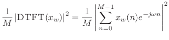
contains ![]() nonzero samples. Then the periodogram is defined as the
squared-magnitude DTFT of
nonzero samples. Then the periodogram is defined as the
squared-magnitude DTFT of ![]() divided by
divided by ![]() [120, p. 65]:7.7
[120, p. 65]:7.7
In the limit as
| (7.24) |
where
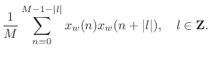
In terms of the sample PSD defined in §6.7, we have
| (7.25) |
That is, the periodogram is equal to the smoothed sample PSD. In the time domain, the autocorrelation function corresponding to the periodogram is Bartlett windowed.
In practice, we of course compute a sampled periodogram
![]() ,
,
![]() , replacing the DTFT with the
length
, replacing the DTFT with the
length ![]() FFT. Essentially, the steps of §6.9
include computation of the periodogram.
FFT. Essentially, the steps of §6.9
include computation of the periodogram.
As mentioned in §6.9, a problem with the periodogram of noise
signals is that it too is random for most purposes. That is,
while the noise has been split into bands by the Fourier transform, it
has not been averaged in any way that reduces randomness, and each
band produces a nearly independent random value. In fact, it can be
shown [120] that
![]() is a random variable whose
standard deviation (square root of its variance) is comparable to its
mean.
is a random variable whose
standard deviation (square root of its variance) is comparable to its
mean.
In principle, we should be able to recover from
![]() a
filter
a
filter
![]() which, when used to filter white noise,
creates a noise indistinguishable statistically from the observed
sequence
which, when used to filter white noise,
creates a noise indistinguishable statistically from the observed
sequence ![]() . However, the DTFT is evidently useless for this
purpose. How do we proceed?
. However, the DTFT is evidently useless for this
purpose. How do we proceed?
The trick to noise spectrum analysis is that many sample power spectra (squared-magnitude FFTs) must be averaged to obtain a ``stable'' statistical estimate of the noise spectral envelope. This is the essence of Welch's method for spectrum analysis of stochastic processes, as elaborated in §6.12 below. The right column of Fig.6.1 illustrates the effect of this averaging for white noise.
Matlab for the Periodogram
Octave and the Matlab Signal Processing Toolbox have a periodogram function. Matlab for computing a periodogram of white noise is given below (see top-right plot in Fig.6.1):
M = 32;
v = randn(M,1);       % white noise
V = abs(fft(v)).^2/M; % periodogram
Next Section:
Welch's Method
Previous Section:
Why an Impulse is Not White Noise


