DAC Zero-Order Hold Models

• Matlab
• Tutorials

As the name indicates, a digital to analog converter (DAC) converts a digital quantity to an analog voltage or current.  But more than this, a DAC converts a discrete-time signal into a continuous-time signal.  The latter operation is almost always accomplished by a zero-order hold (ZOH) function. As we’ll see, it is the ZOH that causes the sinx/x roll-off in the frequency response of the DAC.

This article provides two simple time-domain models of a DAC’s zero-order hold.  These models will allow us to find time and frequency domain approximations of DAC outputs, and simulate analog filtering of those outputs.  Developing the models is also a good way to learn about the DAC ZOH function.  Note:  the models presented here do not include quantization.

Background

Figure 1 is a simplified block diagram of a 4-bit DAC [1].  As shown, a register clocked at sample rate f_sDAC feeds a 4-to-16 decoder that then enables one of 16 analog switches, producing an output voltage that is a fraction of reference voltage V_ref.  This output voltage corresponds to the digital input value.  Although the DAC input is an unsigned value, we will perform all calculations on signed numbers, as explained at the end of the article.

In DSP math, a discrete-time signal is treated as a sequence of impulses of varying amplitudes.  Figure 2 (top) shows an example of a DAC’s discrete-time input signal.  The DAC’s continuous-time output signal is plotted in the middle plot for sample time T = 1/f_sDAC.   As shown, the output signal holds the value of each input sample until the next sample.  This ZOH function occurs because the register output in Figure 1 holds each digital value for one clock cycle.

The impulse response of the DAC’s ZOH function is simply a rectangular pulse of length T, as shown in the bottom of Figure 2.  The frequency response is the continuous Fourier Transform of the rectangular pulse, given by [2]:

$$ H_z(\Omega)= T \, \frac{sin(\Omega T/2)}{\Omega T/2} \,exp(-j\Omega T/2)   \qquad (1) $$

where Ω is continuous radian frequency, and the complex exponential term occurs because the pulse is centered at t = T/2.  H_z(Ω) contains the familiar sinx/x or sinc function.

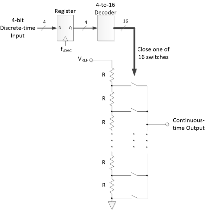
Figure 1.  Simplified block diagram of a 4-bit DAC.

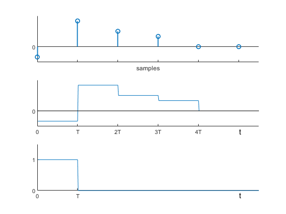
Figure 2.  DAC ZOH function.

Top:  Discrete-time input.  Middle:  Continuous-time output.  Bottom:  ZOH Impulse response.

First Model

For the ZOH function, the input x(n) is a discrete-time signal and the output y(t) is a continuous-time signal, as shown in Figure 3a.  The spectrum of x(n) is unique over a frequency range of 0 to f_sDAC/2, while the spectrum of y(t) is infinite in frequency.  For our model, we’ll consider a limited output frequency range, for example 0 to 4*f_sDAC.  Then we can model the DAC ZOH as a discrete-time system with a sample rate of 8*f_sDAC.

For the first model, we choose to make the impulse response match the continuous-time ZOH function (Figure 2, bottom) at the sample times.  If we let the model have a sample rate of 8*f_sDAC, the block diagram shown in Figure 3b produces the desired impulse response (as we’ll demonstrate in Example 1).   As shown, the model consists of upsampling by 8, followed by an 8-tap boxcar (rectangular) filter.  A simple Matlab function to implement the model is listed below.

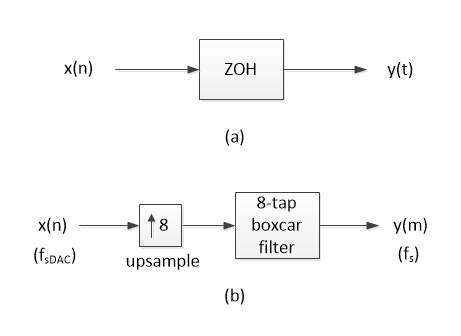
Figure 3.  a) ZOH function.  b) Simple discrete-time model.

First Matlab Model

    %   function y= dac_model(x)  10/30/23    Neil Robertson
    %   Model the zero-order hold (ZOH) function of a DAC
    %
    % x = DAC model input sequence
    % y = DAC model output sequence
    %     sample rate of y is 8 times sample rate of x.
    %
    function y= dac_model(x)
    N= length(x);
    x_up= zeros(1,8*N);
    x_up(1:8:end)= 8*x;          % upsample x by 8
    b= ones(1,8)/8;              % 8-tap boxcar filter
    y= conv(b,x_up);             % filter x_up using b

Example 1.  Impulse Response and Frequency Response

The model’s response to an impulse is a rectangular pulse that is 8 samples long.  The Matlab code to generate the impulse response is simply:

    x= [1 0 0 0];           % impulse input
    y= dac_model(x);        % impulse response

The output y is plotted in the top of Figure 4.  As desired, y matches the ZOH function at the sample times.  The model’s frequency response is the Discrete Fourier Transform of y.  Letting f_sDAC = 1 Hz, we have:

    fs_dac= 1;                % Hz DAC sample rate
    fs= 8*fs_dac;             % Hz sample rate of model output y
    N= 512;                   % DFT length
    k= 0:N-1;                 % frequency index
    f= k*fs/N;                % Hz frequency
    H= fft(y/8,N);            % approx. spectrum due to ZOH
    HdB= 20*log10(abs(H));    % dB magnitude of spectrum

Note we scaled y by 1/8 in taking the FFT.  The dB-magnitude of the response is plotted in the bottom of Figure 4, along with the dB-magnitude of the continuous-time response H_z(f) (from Equation 1).  The model’s response departs from H_z(f) at higher frequencies, but it may be adequate for cases where the frequency range of interest is less than about 2*f_sDAC.  Error is .06 dB at f= f_{s DAC}/2.  Given that y is a sampled version of the continuous-time response, the error can be viewed as due to aliasing.

A usually unwelcome effect of the ZOH magnitude response is roll-off in the frequency response from f = 0 to f_sDAC/2.  As can be seen in the plot, this roll-off is about 4 dB (3.92 dB to be more precise).  The roll-off can be compensated for by using a so-called sinx/x correction filter:  I discussed design of these filters in an earlier post [3].  Also seen in the plot, the peak of the first stopband lobe of |H_z(f)| is -13.26 dB, which occurs at f = 1.43*f_sDAC.

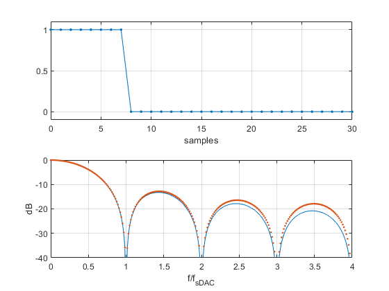
Figure 4.  Top:  Impulse response of first DAC ZOH model.

Bottom:  Magnitude response:  red dots = ZOH model, blue = ZOH

Second Model

As can be seen in Figure 4, the first model’s magnitude response is not very accurate for f greater than 2*f_sDAC.  For an improved model, our goal will be to obtain an accurate magnitude response up to 4*f_sDAC.

We start with the block diagram shown in Figure 5a, where T is the DAC sample time and T_s is the sample time after upsampling by 8.  The input is an impulse, and the output of the boxcar filter is a rectangular pulse of length 8, with duration 7*T_s.  The ZOH shown has hold time of T_s, and the signal at its output is a continuous-time rectangular pulse of length T = 8*T_s   (7*T_s due to the boxcar filter plus T_s of the ZOH).  Thus, the output signal is exactly the impulse response of the DAC ZOH.  The frequency response of the ZOH in Figure 5a has the same form as that of the DAC ZOH, but the hold time is T_s instead of T:

$$ G_z(\Omega)= T_s \, \frac{sin(\Omega T_s/2)}{\Omega T_s/2} \,exp(-j\Omega T_s/2)   \qquad (2) $$

Our approach here will be to find linear-phase FIR filter coefficients b_G whose magnitude response approximates G_z(f) over 0 to f_s/2.  Our model with b_G is shown in Figure 5b.  The model’s overall magnitude response should approximate that of the DAC ZOH.

From the magnitude of G_z(f), we can find b_G by using a Matlab FIR design function such as firpm.  For example, a 15-tap version is as shown:

    b_G= [3 -6 8 -11 17 -36 157 1786 157 -36 17 -11 8 -6 3]/2048;

These coefficients are plotted in the top of Figure 6.  Their frequency response magnitude and the magnitude of G_z(f) are plotted in the bottom of Figure 6.

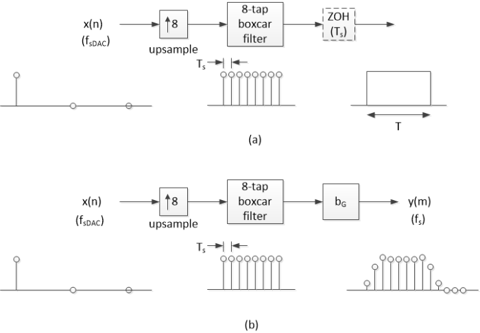
Figure 5.  Derivation of DAC Model with $fs = 8*f_{sDAC}$ (note $1/ f_{sDAC} = T$).

a) Block diagram with zero-order hold of duration $T_s$.

b) Model with approximation of ZOH of duration $T_s$ over 0 to $f_s/2$.

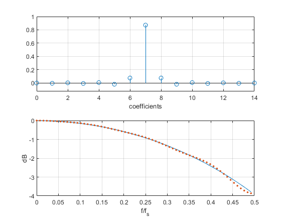
Figure 6.  Top:  Filter coefficients $b_G$.

Bottom:  Red dots = magnitude response of $b_G$,  Blue = Magnitude response of $G_z(f)$.

Matlab Code for this second model, which implements the block diagram of Figure 5b, is listed below.  Figure 7 (top) shows the model’s impulse response, which is slightly modified from a perfect rectangular pulse.  This slight distortion will be made negligible by a subsequent DAC reconstruction filter model, who’s bandwidth must be less than f_s/16 (f_sDAC/2).

The magnitude response is an excellent approximation of the DAC’s ZOH magnitude response, as shown in the bottom plot of Figure 7.  The magnitude response error is .09 dB at 3.15* f_sDAC and -0.2 dB at 3.75* f_sDAC.  Error at f = 0 is .008 dB due to coefficient rounding.  Finally, note that the model’s time delay is greater than the T/2 delay of a DAC’s ZOH.

Second (Improved) Matlab Model

    % function y= dac_model_2(x)   10/30/23 Neil Robertson
    % Model the zero-order hold (ZOH) function of a DAC
    %
    % x = DAC model input sequence
    % y = DAC model output sequence
    %     sample rate of y is 8 times sample rate of x.
    %
    function y= dac_model_2(x)
    N= length(x);
    x_up= zeros(1,8*N);
    x_up(1:8:end)= 8*x;              % upsample x by 8
    % b_G is a FIR with freq response approximating Gz
    b_G= [3 -6 8 -11 17 -36 157 1786 157 -36 17 -11 8 -6 3]/2048;
    b_box= ones(1,8)/8;              % 8-tap boxcar filter
    b= conv(b_G,b_box);              % overall response
    y= conv(b,x_up);                 % filter x_up using b

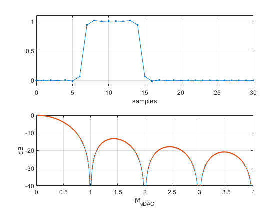
Figure 7.  Top:  Impulse response of second DAC ZOH model.

Bottom:  Magnitude response.  Red dots = ZOH model, blue = ZOH.

Example 2.  Sinusoidal Input

The following Matlab code generates a sinewave with sample rate of 100 Hz and frequency f₀ = 15 Hz.  It then uses dac_model_2 to find the output y of the DAC ZOH and computes the power spectral density (PSD) over f = 0 to 4*f_sDAC (0 to 400 Hz).  The function psd_kaiser is listed in the appendix of the PDF version.

    fs_dac= 100;         % Hz DAC sample rate
    T= 1/fs_dac;         % s DAC sample time
    fs= fs_dac*8;        % Hz ZOH model sample rate
    % create sine at 15 Hz
    f0= 15;              % Hz sine frequency
    N= 256;
    n= 0:N-1;
    x= sin(2*pi*f0*n*T);     % sine signal
    y= dac_model_2(x);       % DAC model output signal
    [PdB,f]= psd_kaiser(y,1024,fs);    % spectrum of DAC output

The output signal y is shown in Figure 8 (top), where the effect of the ZOH is visible as “stair steps”, like those in the middle plot of Figure 2.  The spectrum of y is shown in the bottom of Figure 8.  Since the discrete-time signal x has a sample rate of 100 Hz, images appear at 100 +/- 15 Hz, 200 +/- 15 Hz, etc.  These images have been attenuated by the DAC ZOH magnitude response, which is also shown in the plot.  The level of the images decreases only gradually with frequency due to the slow roll-off of the ZOH response.  To obtain a sinewave, the images must be attenuated using a DAC reconstruction filter, as discussed in the next example.

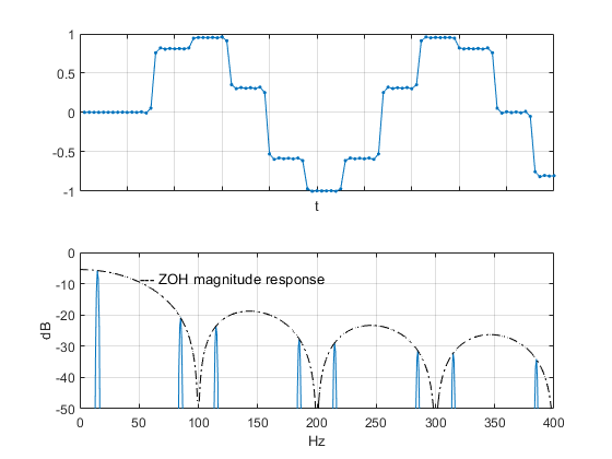
Figure 8.  Top:  DAC ZOH model output y(1:100) for input x = 15 Hz sinewave, f_{s_dac} = 100 Hz.

Bottom:  Spectrum of model output.

Example 3.  Modeling a DAC Reconstruction Filter

As mentioned, a DAC reconstruction filter is needed to attenuate the images in the DAC’s output spectrum.  We can add a model of a continuous-time reconstruction filter to our ZOH model, as shown in Figure 9.  To create an accurate Infinite Impulse Response (IIR) model of an ideal continuous-time filter, we use the impulse-invariant method, as I discussed in an earlier post [4].  It is also possible to model a lossy continuous-time filter [5].  We need to be careful when using the IIR filter model.  The sample frequency of the model is much higher than the filter cutoff frequency, which causes the filter poles to lie close to the unit circle in the z-plane.  Be aware that truncating the coefficient values may move the pole locations only slightly, yet cause bad distortion to the filter response.

As a reconstruction filter for the 15 Hz sine of Example 2, we’ll use a 5^th order Butterworth lowpass filter with cutoff frequency of 30 Hz.  The coefficients of an IIR ideal filter model for sample rate = 8*f_sDAC = 800 Hz are listed below.  We calculated the ZOH output y in the previous example.  The IIR filter output u for input y is calculated using the Matlab filter function, as shown.

    % Impulse invariant DAC recon filter model [4]
    % 5th order Butterworth, fc= 30 Hz, fs= 800 Hz.
    b= .0001*[0 .2593 2.4408 2.0958 .1641];
    a= [1 -4.2402 7.2415 -6.2213 2.6870 -.4665];
    u= filter(b,a,y);          % output of DAC recon filter

The spectrum at the ZOH output for the 15 Hz sinewave is shown in the top plot of Figure 10, and the frequency response magnitude of our Butterworth filter model is shown in the middle plot.  The spectrum at the filter output, with attenuated images, is shown in the bottom plot.  Figure 11 plots the ZOH time-domain output y, along with the output u of the Butterworth filter, which is, as hoped, a sinewave.

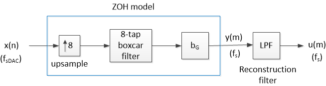
Figure 9.  DAC ZOH model with reconstruction filter model.

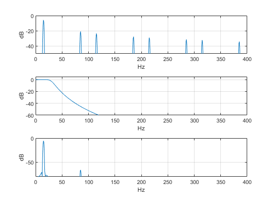
Figure 10.  Top:  Spectrum of DAC ZOH model output, signal = 15 Hz sine, f_{s_dac} = 100 Hz.

Middle:  Magnitude response of DAC reconstruction filter, f_c = 30 Hz.

Bottom:  Spectrum magnitude at output of reconstruction filter model.

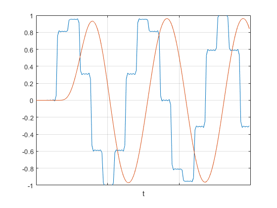
Figure 11:  Blue:DAC ZOH model output y(1:150), signal = 15 Hz sine, f_{s_dac} = 100 Hz.

Red:  Output u(1:150) of reconstruction filter model.

Signed and Unsigned Signals

Although the DAC input is unsigned, we have performed all calculations on signed numbers.  Why is this valid?  DSP calculations are performed using two’s-complement (signed) binary numbers.  These values are converted to unsigned binary numbers for the DAC by inverting the MSB, as indicated in Figure 12.  As shown, the positive-voltage DAC output r can be converted to the bipolar signal y = r - V_ref /2. (The unipolar to bipolar converter can be simply an ac-coupling capacitor for signals with no DC component).  For a 4-bit input, the signals have the following ranges, where we let V_ref = 1.0 volts (See Figure 1):

x                  1000 to 0111 = -8/16 to 7/16 (fraction of full-scale)

u                  0000 to 1111 = 0 to 15/16

r                   0 to 15/16 volts

y = r – ½     -8/16 to 7/16 volts

The voltage output y has the same values as the two’s-complement input x.  So, for convenience, we can ignore the conversions and perform all calculations as signed.

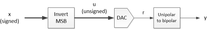
Figure 12.  Signed and unsigned signals.

For Appendix, see PDF version.

References

1.  Kester, Walt, “Basic DAC Architectures 1”, Analog Devices, Rev A., October, 2008,

https://www.analog.com/media/en/training-seminars/tutorials/MT-014.pdf

2.  Mitra, Sanjit K., Digital Signal Processing, 2^nd Ed., McGraw-Hill, 2001, p 348 – 349.

3.  Robertson, Neil, “Design a DAC sinx/x Corrector”, DSPrelated.com, July, 2018, https://www.dsprelated.com/showarticle/1191.php

4.  Robertson, Neil, “Modeling Anti-Alias Filters”, DSPrelated.com, Sept., 2021,

https://www.dsprelated.com/showarticle/1418.php

5.  Robertson, Neil, “Simple Discrete-Time Modeling of Lossy LC Filters”, DSPrelated.com, April, 2023,

https://www.dsprelated.com/showarticle/1507.php

6.  Robertson, Neil, “A Simplified Matlab Function for Power Spectral Density”, DSPrelated.com, March, 2020, https://www.dsprelated.com/showarticle/1333.php

Neil Robertson      January, 2024

Sign in