The Discrete Fourier Transform and the Need for Window Functions

• Matlab
• DFT_FFT
• Tutorials

The Discrete Fourier Transform (DFT) is used to find the frequency spectrum of a discrete-time signal.  A computationally efficient version called the Fast Fourier Transform (FFT) is normally used to calculate the DFT.  But, as many have found to their dismay, the FFT, when used alone, usually does not provide an accurate spectrum.  The reason is a phenomenon called spectral leakage.

Spectral leakage can be reduced drastically by using a window function in conjunction with the DFT.  In this article, we’ll see why spectral leakage occurs, then we’ll introduce window functions and show how they improve the spectrum.

For a discrete-time sequence x(n), the DFT is defined as:

$$ X(k)= \sum_{n=0}^{N-1} x(n)e^{-j2\pi kn/N} \qquad (1) $$

where

X(k) = discrete frequency spectrum of time sequence x(n)

N = number of samples of x(n) and X(k)

n = time index = 0: N-1

k = frequency index

We see that by definition, the DFT applies to a finite-length signal of N samples.  For sample time of T_s, the discrete-time variable is given by:

t = nT_s                           (2)

For sample frequency f_s = 1/T_s, the discrete frequency variable is given by:

f = k*f_s/N                       (3)

In general, X(k) is complex.  For real x(n), the real part of X(k) is even with respect to f = f_s/2, and the imaginary part is odd.

The DFT is able to compute a spectrum of any signal whose duration is N samples or less.  Since many signals that we are interested in don’t have a nicely defined start and end, we end up using a segment of the signal of length N to compute the DFT.  As an example, consider sinewaves of 8 or 9 Hz, sampled at f_s = 128 Hz.  We’ll let N = L = 64 samples, where we use L in place of N for convenience in subsequent developments.  Matlab code to create an 8 Hz sinewave and compute its DFT is listed below, where we use the Matlab function fft to compute the DFT of Equation 1.  The function computes L values of the discrete spectrum, i.e., k = 0: L-1.

    fs= 128;                     % Hz sample frequency
    Ts= 1/fs;                    % s sample time
    L= 64;                       % total number of samples
    f0= 8;                       % Hz sine frequency
    n= 0:L-1;                    % time index
    x= sin(2*pi*f0*n*Ts)*2/L;    % discrete-time sinusoid
    X = fft(x,L);                % discrete spectrum via DFT
    Xmag= abs(X);                % magnitude of X
    k= 0:L-1;                    % frequency index
    f= k*fs/L;                   % Hz discrete frequency

Here, we have scaled the sine amplitude by 2/L in order to obtain a magnitude of the spectral components of 1.0.  Note that for the complex vector X, the Matlab function abs computes the magnitude of each element of X.

The discrete-time sinusoid x(n) is plotted in the top of Figure 1, where we see that there are exactly four cycles of the sinewave in 64 samples. The DFT is plotted in the middle for discrete frequencies from 0 to f_s.  X(k) is pure imaginary, which occurs because x(n) is an odd function. The bottom plot shows the magnitude of X(k), plotted over 0 to f_s/2. As dictated by Equation 3, the discrete frequencies or bins are spaced f_s/L = 2 Hz. The plot shows a single spectral component at 8 Hz.

So far, so good. But now let’s try the same Matlab code at a different sine frequency:

    f0= 9;    % Hz

The sinusoid is plotted in the top of Figure 2, where there are now 4.5 cycles in 64 samples.  The magnitude of X(k) is plotted in the bottom plot.  The ugly-looking spectrum is spread over many bins:  this is the aforementioned spectral leakage phenomenon.  Looking at the frequency axis, we see an obvious problem:  there is no bin at 9 Hz.  As we’ll see, there is no perfect fix for this problem, but we can improve things.

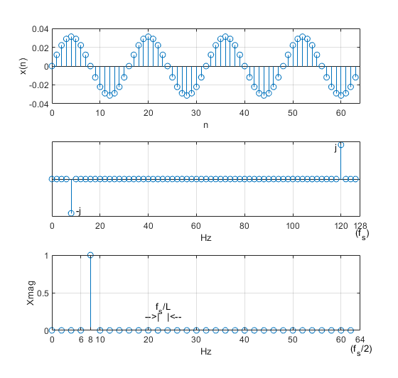
Figure 1.  DFT of a sinusoid.  f₀ = 8 Hz, f_s = 128 Hz, L = 64 samples.

Top: Discrete-time sinewave.   Middle: X(f) for f = 0 to f_s.   Bottom: |X(f)| for f = 0 to f_s/2.

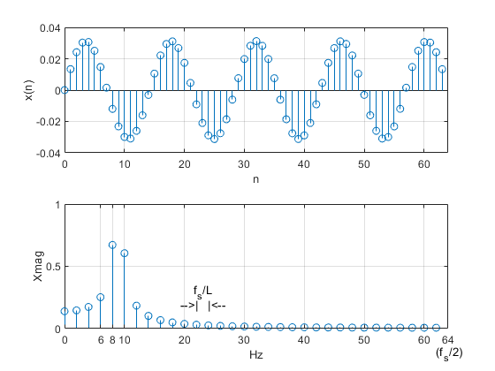
Figure 2.  DFT of a sinusoid.  f₀ = 9 Hz, f_s = 128 Hz, L = 64 samples.

Top: Discrete-time sinewave.   Bottom: |X(f)| for f = 0 to f_s/2.

An Inconvenient Window

Figure 3 provides a view of capturing L samples of a sinewave.  The top plot shows samples of the sinewave.  The middle plot shows a rectangle function that has L = 64 samples equal to 1.0.  The bottom plot shows the result when we multiply the sinewave by the rectangle function on a sample-by-sample basis.

Basically, we are opening a window that captures L samples of the sinewave, and the window is just a rectangle function.  Windowing occurs whenever the duration of the captured signal exceeds t = L*T_s, which is very often the case for real-world signals.  Mathematically, windowing is element-by-element multiplication of the sinewave by the window function – that is, modulation of the sinewave by the window function.

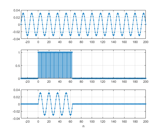
Figure 3.  Windowing by the rectangular window function.

Top: sinewave to be captured.   Middle: rectangular window function.   Bottom: windowed sinewave.

When using the DFT, we can see the effect of the rectangular window more clearly by keeping the zero-padding at the end of the sinewave (zero-valued samples above n = 63 in Figure 3).  This will give us a smaller discrete frequency step of fs/N, where N is the total number of samples, including zero-padding.

The following Matlab code generates 64 samples of a sinewave as before, with f₀ = 8 Hz.  Then zeros are appended to obtain a total of 8*64 = 512 samples.  We then find the DFT of this zero-padded signal.  (Note:  although we explicitly append zeros here, the Matlab FFT function will automatically zero-pad the signal x if length of x is less than N).

    fs= 128;                     % Hz sample frequency
    Ts= 1/fs;                    % s sample time
    L= 64;                       % number of sinewave samples
    f0= 8;                       % Hz sine frequency
    n= 0:L-1;                    % time index
    u= sin(2*pi*f0*n*Ts)*2/L;    % discrete-time sinusoid
    R= 8;                        % zero-padding factor
    N= R*L;                      % total samples with zero-padding
    x= [u zeros(1,N-L)];         % zero-padded signal
    X = fft(x,N);                % discrete spectrum via DFT
    Xmag= abs(X);                % magnitude of X
    k= 0:N-1;                    % frequency index
    f= k*fs/N;                   % Hz discrete frequency

The zero-padded signal x is plotted in the top of Figure 4, and the magnitude of the spectrum X is plotted in the bottom, where we are limiting the frequency axis to 0 to 32 Hz (f_s/4).  Spectral components due to the modulation of the sinewave by the rectangular window that were not seen in Figure 1 are now visible. (The components of the L-point DFT of Figure 1 are indicated by the blue circles). The spectrum near 8 Hz is spread out by the modulation, and there are sidelobes.  We also see that in this special case where the sine’s spectrum falls exactly on a bin, the components at the other bins of the L-point DFT are zero.

Now let

    f0= 9; % Hz

The zero-padded signal x is plotted in the top of Figure 5, and the magnitude of the spectrum X is plotted in the bottom.  We can now see that the spectral leakage components of Figure 2 all fall at sidelobe peaks of the spectrum.Furthermore, the amplitude of the sidelobes of Xmag decreases very slowly with frequency.  Basically, the rectangular window has made a mess of the spectrum!

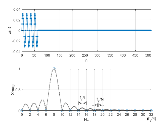
Figure 4. Rectangular windowing of sinewave, with zero-padding. f₀ = 8 Hz, f_s = 128 Hz

Top: Windowed sinewave with zero padding.

Bottom: Magnitude spectrum of windowed sinewave.

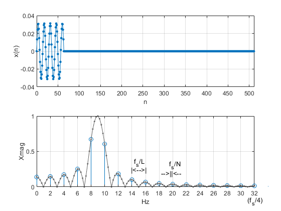
Figure 5. Rectangular windowing of sinewave, with zero-padding. f₀ = 9 Hz, f_s = 128 Hz

Top: Windowed sinewave with zero padding.

Bottom: Magnitude spectrum of windowed sinewave.

Spectrum of the Rectangular Window

Figures 4 and 5 showed the spectra of windowed sinusoids. Now let’s find the spectrum of the rectangular window itself.

The following Matlab code generates a window of L= 64 ones, then appends zeros to obtain a total of N = 8*64 = 512 samples, as shown in the top plot of Figure 6. We find the DFT magnitude Xmag of this zero-padded rectangular window, then we swap the left and right halves of Xmag to obtain a spectrum centered at 0 Hz. We plot this shifted magnitude response with frequency units of f_s/L in the bottom plot of Figure 6.

    fs= 1;                    % Hz sample frequency
    L= 64;                    % length of rectangular window
    R= 8;                     % zero-padding factor
    N= R*L;                   % total samples with zero-padding
    x= [ones(1,L) zeros(1,N-L)]/L;    % rectangular window with zero padding
    X = fft(x,N);             % discrete spectrum via DFT
    Xmag= abs(X);             % magnitude of X
    k= 0:N-1;                 % frequency index
    f= k*fs/N;                % Hz frequency
    % spectrum centered at 0 Hz
    Xmag_shift = fftshift(Xmag);    % swap right half and left half of Xmag
    f_shift= f- fs/2;               % shift freq range to -fs/2:fs/2

The functional form of the spectrum magnitude plotted in the bottom of Figure 6 is given by:

$$|X(k)|= \left|\frac{sin(\pi kL/N)}{sin(\pi k/N)}\right| \qquad (4) $$

where k is the frequency index, L is the length of the window, and N is the length of x, including zero padding.  See Appendix A in the PDF version for a derivation of equation 4. The rectangular window’s spectrum has large sidelobes that decay slowly with frequency.  As we have seen, these unwanted sidelobes appear on the spectrum of our sinewaves. The sidelobes look even worse when plotted on a dB magnitude scale, as we’ll see.  Finally, note that the mainlobe bandwidth is inversely proportional to L:  null-null bandwidth = 2*fs/L.

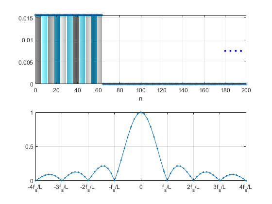
Figure 6.  Spectrum of the rectangular window.

Top: Zero-padded window.   Bottom: Spectrum magnitude centered at 0 Hz.

Comparing Figure 4 or 5 with Figure 6, you may wonder why, given that the window spectrum of Figure 6 is symmetrical, the spectrum of the windowed sinewave is not.  If multiplication (modulation) in the time domain is equivalent to convolution in the frequency domain, shouldn’t the convolution of the window with a single spectral component be symmetrical?  This would be the case for continuous-time signals, but for discrete-time signals, the rule is:  “multiplication in the time domain is equivalent to circular convolution in the frequency domain”.  Basically, the convolution components that would fall outside the range of 0 to f_s under linear convolution wrap-around and add to the spectrum under circular convolution, causing the asymmetry seen in Figures 4 and 5.  See Appendix B in the PDF version for further details.

Improved Spectrum using Window Functions

Given that the rectangular window has such a deleterious effect on the DFT, we ask:  is there any way to improve things?  There is, and it involves changing the shape of the window.  We desire a window that has a more confined spectrum than the rectangular window.

The top of Figure 7 plots samples of a sinewave, as was shown in Figure 3.  The middle plot shows a window function with L = 64 samples that has a smooth shape whose amplitude starts and ends near zero.  The bottom plot shows the result when we multiply the sinewave by the window function on a sample-by-sample basis.  The idea is to multiply the signal by this window, then take the DFT.  At first blush, this looks like a drastic operation; after all, we’re attenuating a large portion of the L samples.  But it is less drastic than the abrupt chopping done by the rectangular window. 

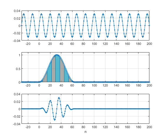
Figure 7.  Windowing by a smooth window function.

Top: sinewave to be captured.   Middle: window function.   Bottom: windowed sinewave

The window function shown in Figure 7 is the often-used Hann, or Hanning window, and is given by [1]:

$$ w(n)= 0.5(1-cos(2\pi n/L)),\; n= 0:L-1 \qquad(5)$$

As an example, for L = 8, we have:  

w = [0  0.1464  0.5  0.8536  1  0.8536  0.5  0.1464].  

Note that Equation 5 is implemented by the Matlab function hann(L,’periodic’).

Let’s find the spectrum of a sinewave using the Hanning window.  Again, we’ll use a 9 Hz sinewave of length L = 64 samples, with f_s = 128 Hz.  In the following Matlab code, we create a Hanning window of length L, then multiply the sine with the window on a sample-by-sample basis (The Matlab operator .* performs this operation).  We then zero-pad the windowed sinewave u to obtain the signal x with total length of 512 samples (The factor of 2 in the computation of x scales the spectrum magnitude for a maximum value of 1.0).  The windowed, zero-padded sinewave x is shown in the top of Figure 8.  Keep in mind that the zero-padding shown is used to increase the frequency resolution of the spectrum, but is not a requirement for computing the DFT.  Finally, we take the DFT of x.  The resulting spectrum magnitude is shown in the bottom of Figure 8, where we are limiting the frequency axis to 0 to 32 Hz (f_s/4).

    fs= 128;                      % Hz sample frequency
    Ts= 1/fs;                     % s sample time
    f0 = 9;                       % Hz sine frequency
    L= 64;                        % length of window
    R= 8;                         % zero-padding factor
    N= R*L;                       % total samples with zero-padding
    n= 0:L-1;                     % time index prior to zero padding
    win= .5*(1-cos(2*pi*n/L));    % hanning window of length L
    u= sin(2*pi*f0*n*Ts)*2/L;     % discrete-time sine
    u_win= win.*u;                % windowed sine
    x= 2*[u_win zeros(1,N-L)];    % windowed, zero-padded sine
    X = fft(x,N);                 % discrete spectrum via DFT
    Xmag= abs(X);                 % magnitude of X
    k= 0:N-1;                     % frequency index
    f= k*fs/N;                    % Hz frequency

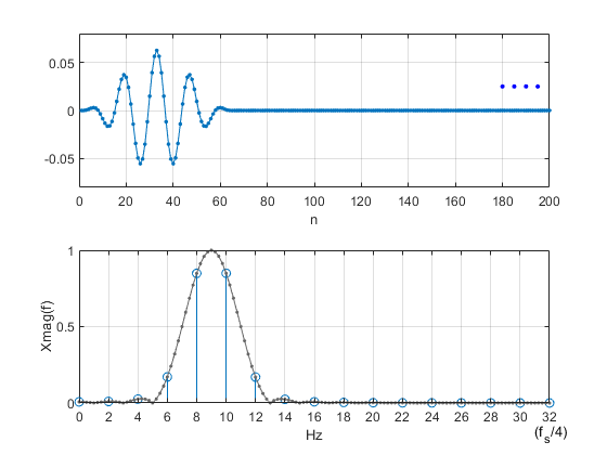
Figure 8.  Hanning windowed sinewave, with zero-padding.  f₀ = 9 Hz, f_s = 128 Hz

Top: Windowed sinewave with zero padding.

Bottom: Magnitude spectrum of windowed sinewave.

Comparing the spectrum of Figure 8 to that of figure 5, we see that the sidelobes are much lower.  However, we still have the spectrum near 9 Hz spread-out due to modulation by the window function (it’s even somewhat wider than for the rectangular window).  Unfortunately, this is the case for any window function.

We can plot the two spectra on a dB scale using:

    XdB= 20*log10(Xmag);

The dB spectra are shown in Figure 9.  Again, the spectrum labeled “rectangular” is what you get if you just take the DFT of the captured sinewave:  it is the spectrum of a sinewave that is modulated by a rectangular window function.  The spectrum labeled “Hanning” results from modulating the sinewave with a Hanning window before taking the DFT.  As already mentioned, using the Hanning window has greatly improved the sidelobes, but the main lobe is annoyingly wide, with a -3 dB bandwidth of almost 3 Hz.  Note, though, that mainlobe bandwidth is inversely proportional to L.  So, at the price of increasing L, we can decrease this bandwidth.  For example, Figure 10 plots the windowed sinewave spectra for f₀ = 9.25 Hz and L = 256.  The Hanning window case now looks somewhat more like an ideal sine spectrum.

One lesson we have learned can be stated as follows:  suppose you captured an unknown signal, took the zero-padded DFT with a Hanning window, and got a spectrum that looked like Figure 10.  You might be tempted to think that the sidelobes seen in the plot were a feature of the signal itself.  But we now know that the sidelobes are due to the window function.

The spectra of Figure 10 used zero-padding with a DFT length N = 8*L.  Zero-padding is not necessary to obtain a valid spectrum:  for example, Figure 11 shows the spectra with no zero padding.  Here, L = N = 256, and discrete frequency step f_s/L = 128/256 = 0.5 Hz (thus, our choice of f₀ = 9.25 Hz falls halfway between discrete frequency bins).  Note that the peaks of both spectra are lower that the peaks for the cases with zero-padding.  This occurs because f₀ falls on a frequency bin for the zero-padded case, but not for the non-zero-padded case.  Finally, we should keep in mind that the skirts of the response are points on the sidelobes of Figure 10.

Comparing the spectra of the window functions themselves, Figure 12 plots the dB spectra of the rectangular and Hanning functions, centered at 0 Hz.  Both functions have bandwidth inversely proportional to L.  The two most important properties of a window function are bandwidth (i.e., noise bandwidth) and sidelobe level.  The rectangular window has very high sidelobes that fall off rather slowly vs. frequency (first sidelobe at -13 dB from main lobe).  The Hanning window has lower sidelobes (first sidelobe at -31.5 dB), but wider bandwidth.  In general, window functions with lower sidelobe level have wider bandwidth.  Sidelobe level is particularly important when trying to display a small signal in the presence of a large signal at a different frequency.  I discussed window function properties in an earlier post [2].  (Note this earlier post used different definitions of the quantities N and L).

There are many window functions with lower sidebands than the Hanning window [3].  The Kaiser window has adjustable sidelobe level; I discussed it briefly in an earlier post [4].

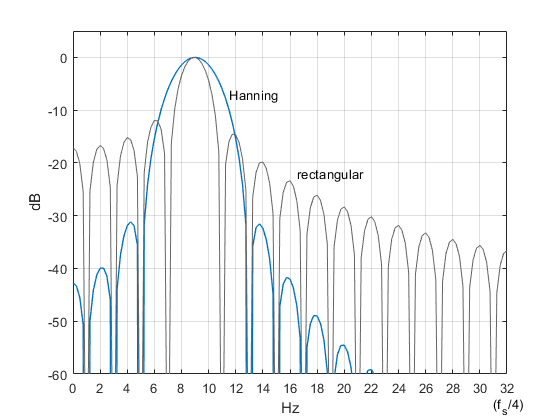
Figure 9.  Spectra of sinewaves using Hanning and rectangular windows.

f₀ = 9 Hz, f_s = 128 Hz, L= 64, N = 8*L = 512.

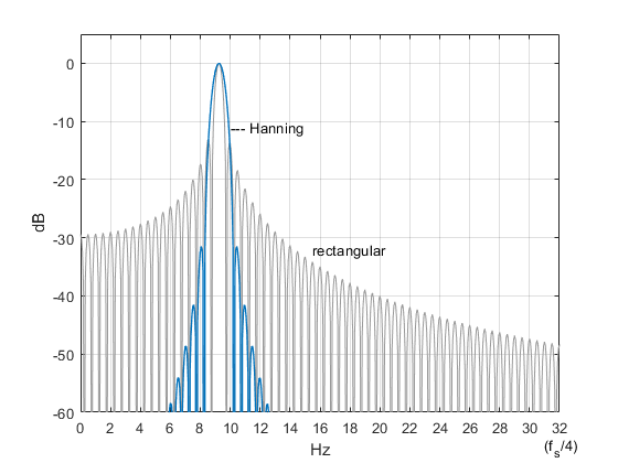
Figure 10.  Spectra of sinewaves using Hanning and rectangular windows.

f₀ = 9.25 Hz, f_s = 128 Hz, L= 256, N = 8*L = 2048.

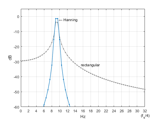
Figure 11.  Spectra of sinewaves using Hanning and rectangular windows.

f₀ = 9.25 Hz, f_s = 128 Hz, L = N = 256 (no zero-padding).

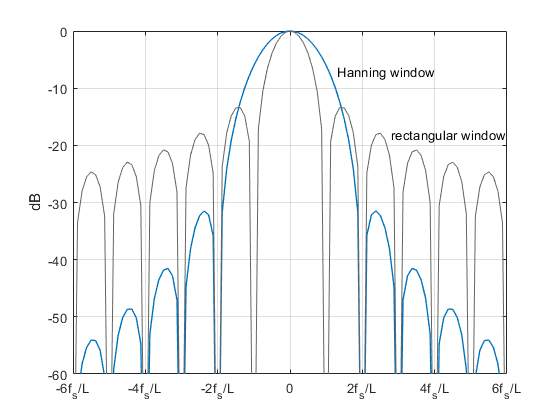
Figure 12.  Spectra of Hanning and rectangular windows.

For appendices, see the PDF version of this article.

References

1.  Lyons, Richard, Understanding Digital Signal Processing, Third Ed., Prentice Hall, 2011, p 91.

2.  Robertson, Neil, “Evaluate Window Functions for the Discrete Fourier Transform”, dspRelated website, Dec., 2018, https://www.dsprelated.com/showarticle/1211.php

3.  Wikipedia article on Window Functions, https://en.wikipedia.org/wiki/Window_function

4.  Robertson, Neil, “A simplified Matlab Function for Power Spectral Density”, dspRelated website, March, 2020, https://www.dsprelated.com/showarticle/1333.php

5.  Lyons, Appendix B.

6.  Courant, Richard and Robbins, Herbert, What is Mathematics?, Oxford University Press, 1996, p 65.

7.  Mitra, Sanjit K., Digital Signal Processing, Second Ed., McGraw-Hill, 2001, Table 3.5.

Neil Robertson   November, 2021

Sign in