Modeling Anti-Alias Filters

• Matlab
• Tutorials

Digitizing a signal using an Analog to Digital Converter (ADC) usually requires an anti-alias filter, as shown in Figure 1a.  In this post, we’ll develop models of lowpass Butterworth and Chebyshev anti-alias filters, and compute the time domain and frequency domain output of the ADC for an example input signal.  We’ll also model aliasing of Gaussian noise.  I hope the examples make the textbook explanations of aliasing seem a little more real.  Of course, modeling of the anti-alias filter is often not a necessity.  It may be adequate to simply verify that the filter has enough stopband attenuation at the unwanted frequencies and acceptable passband performance.

The anti-alias filter is a continuous-time (analog) device, so to model the filtering and aliasing process, we need to model the analog filter H(s) using a discrete-time filter G(z) that has approximately the same frequency response.  This will allow us to examine the effect of aliases, and model passband imperfections, such as ripple and non-flat group delay.  We’ll use the approach shown in Figure 1b.  The model consists of G(z), followed by downsampling by R, then quantization.  G(z) thus has a sample rate of R times the ADC sample rate f_sadc.  R is an integer greater than or equal to 2.

Figure 2a shows an example spectrum of the input signal x, along with the magnitude response of the anti-alias filter.  As shown, x has several frequency components.  Figure 2b shows the filtered signal at the ADC input.  The spectral components at the ADC input can be classified by Nyquist zone [1], where each Nyquist zone has a range of 0.5*f_sadc, starting at 0 Hz.  Signals above the first Nyquist zone produce aliases:  a frequency component at f₀ produces aliases at frequencies:

$$ f= |kf_{sadc} \pm f_0|,\,k= 1,2, ... \qquad (1) $$

where f_sadc is the sample rate of the ADC.  We’re interested in any alias that falls in the first Nyquist zone.  Figure 2c shows the aliases of the component at f_h.

Now consider the digital filter G(z).   Since we are trying to model an analog anti-alias filter, we must minimize aliasing of any significant frequency component in the digital model.  For our example signal, the highest-frequency significant component occurs at f_h, which is in the 3^rd Nyquist zone.  This zone extends to 1.5*f_sadc.  So, in this case, we can prevent aliasing of this component in the digital filter by operating the digital filter at twice this rate, or 3*f_sadc.  If a component at the output of H(s) is at a sufficiently low level, it can be omitted from the simulation:  e.g., the component shown at f_x.  The model of Figure 1b produces significant aliases only in the downsample-by-R block, which models the sampling process of the ADC.  In this example, R = 3.  We have assumed that the ADC frequency response is flat up to f_h.

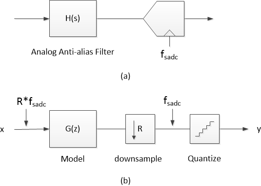
Figure 1.  a) ADC with anti-alias filter.  b) Discrete-time Model using digital filter and downsampling.

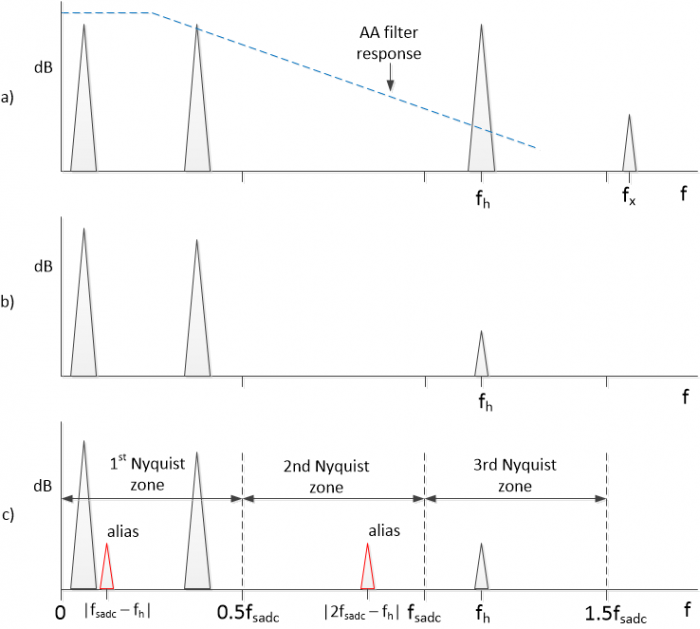
Figure 2.  Example signal spectra. a) at input to anti-alias filter, with anti-alias filter magnitude response.     b) at output of anti-alias filter.  c) ADC Nyquist zones, showing aliases.

The next task is to find a model G(z) for a given anti-alias filter.  In this article, we’ll consider Infinite Impulse Response (IIR) Butterworth and Chebyshev lowpass filters.  I provide two short Matlab functions that generate the filter coefficients (see Appendices A and B of the PDF version).  If you need to model elliptic filters, try the Matlab function ellip.  Note that we won’t be modelling ADC impairments.

Filter Models

Anti-alias filters can take many forms, some of which are easier to model than others.  Here, we’ll limit ourselves to Butterworth or Chebyshev lowpass filters.  We’ll make the simplifying assumption that the modeled analog filters have ideal responses.  Thus, we are not taking into account component value error, Q, stray inductance, or stray capacitance.  We need to be aware that these factors can be significant for high-order filters or at RF frequencies, reducing the accuracy of the model.  There is a brief discussion of LC analog filter design in Appendix D of the PDF version.

We’ll use the s-plane poles of the analog filter to find the coefficients of our filter model G(z).  There are two main methods for generating G(z):  bilinear transform and impulse invariance [2].  For an anti-alias filter, we care about accuracy of both the passband and stopband of the model.  After all, the level of the aliased signals depends on the filter stopband.  It turns out that the impulse invariance method gives a more accurate model.

As an example, the magnitude response an ideal analog Butterworth filter of order N is given by [3]:

$$ |H(j\omega)|=\frac{1}{\sqrt{1+\omega^{2N}}}\qquad (2) $$

where ω is radian frequency.  Figure 3 plots an example 5^th-order Butterworth magnitude response, along with |G(z)| using the bilinear transform and impulse invariance methods.  Clearly, impulse invariance is the best choice for modeling the stopband, but it’s not perfect:  the model response departs from the analog response for f > 40 Hz or so in this example.

We’ll use two simple Matlab functions that employ impulse invariance: butter_impinvar (Appendix A of the PDF version) generates coefficients for Butterworth filter models and cheby_impinvar (Appendix B) generates coefficients for Chebyshev filter models.  Both of these functions rely on the Matlab impulse-invariant digital filter synthesis function impinvar, which I discussed in an earlier post [4].

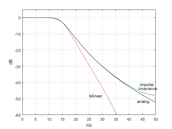
Figure 3.  Magnitude response of ideal 5^th order analog Butterworth filter and discrete-time approximations.  f_c = 15 Hz and f_s = 100 Hz.

Example 1.  A Butterworth anti-alias filter

In this example, we’ll model a 5^th order Butterworth anti-alias filter with multiple sinusoidal inputs, with the highest frequency input at 85 Hz and f_sadc = 100 Hz.  85 Hz is in the 2^nd Nyquist zone, so we can avoid aliases in the filter model by using f_s = 2*f_sadc.  For simplicity, we’ll ignore ADC quantization in this example.

Here are the simulation parameters:

Filter model f_c = 25 Hz

Filter order = 5

f_sadc = 100 Hz

R= 2

Filter model f_s = R*f_sadc = 200 Hz

Input signal:  three equal-level sines at 5, 40, and 85 Hz.

We will compute spectra of the input signal, filter output, and ADC output.  Keep in mind that the simulation computes the discrete-time output y, which could also be used in a time-domain simulation (e.g., receiver interference simulation).  The Matlab code to simulate the filter is as follows.  The function butter_impinvar(order,fc,fs) computes the digital filter coefficients, given order, -3 dB frequency, and sample frequency.  The function’s code is listed in Appendix A of the PDF version.  The code for the function psd_kaiser is listed in Appendix C.

    fc= 25;                    % filter -3 dB frequency
    fsadc= 100;                % Hz ADC sample rate
    R= 2;                      % downsample ratio
    fs= R*fsadc;               % Hz filter sample rate
    Ts= 1/fs;
    f0= 5; f1= 40; f2= 85;     % Hz sine frequencies
    A= sqrt(2);                % V sine amplitude
    N= 2048;                   % number of samples
    n= 0:N-1;                  % sample index
    % input signal
    x= A*sin(2*pi*f0*n*Ts) + A*sin(2*pi*f1*n*Ts) + A*sin(2*pi*f2*n*Ts);
    % find 5th-order digital Butterworth filter coeffs.
    order = 5;
    [b,a]= butter_impinvar(order,fc,fs);
    %            
    u= filter(b,a,x);                 % compute output of filter
    y= u(1:R:end);                    % downsample by R
    % spectra of x, u, and y
    [PdB1,f]= psd_kaiser(x,N,fs);     % spectrum of input signal
    [PdB2,f]= psd_kaiser(u,N,fs);     % spectrum at output of filter
    [PdB3,f2]= psd_kaiser(y,round(N/R),fsadc);   % spectrum at output of ADC
    % filter response
    [h,f3]= freqz(b,a,256,fs);
    H= 20*log10(abs(h));               % dB magnitude response

Simulation results are shown in Figure 4.  Since f_sadc = 100 Hz, any component above 50 MHz will produce an alias.  At the output of the filter (Figure 4c), the component at 85 Hz has amplitude of about -56 dB.  After downsampling, this aliases to 15 Hz, as seen in Figure 4d.

Finally, note that the filter model in this example has a few dB of error in the stopband response for input frequencies between 95 and 100 Hz.  If we had frequencies in that range, we could obtain more accuracy by using f_s = 3*f_sadc (R = 3).

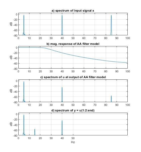
Figure 4.  5^th order Butterworth anti-alias filter with sinusoidal inputs.  f_sadc = 100, R = 2.

a) Input spectrum of anti-alias filter.  b) Magnitude response of Anti-alias filter model.

c) Spectrum at output of anti-alias filter.  d) Spectrum at output of ADC.

Chebyshev Response

For a given filter order, either a Butterworth or Chebyshev analog filter uses the same number of components, but a Chebyshev filter has better stopband attenuation.  The price you pay for the improved stopband attenuation is ripple in the passband.  While a Butterworth filter is defined by order and cutoff (-3 dB) frequency, a Chebyshev filter is defined by order, passband ripple in dB, and either ripple band edge frequency f_r or cutoff frequency f_c.

Figure 5 compares the response of 5^th order Butterworth and Chebyshev analog filters, each with f_c = 15 Hz.  The Chebyshev filter has passband ripple of 0.1 dB.  Figure 5a shows the improved stopband attenuation of the Chebyshev filter, while Figure 5b shows the passband ripple of the Chebyshev compared to the maximally flat Butterworth.  Finally, Figure 5c compares group delay.  Although the 0.1 dB Chebyshev has a large peak in group delay, the group delay flatness over most of the passband is similar to that of the Butterworth filter.

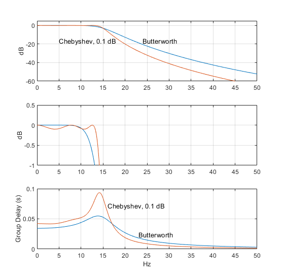
Figure 5.  0.1 dB Chebyshev and Butterworth 5^th order analog filters with f_c = 15 Hz

a) Magnitude responses.

b) Magnitude responses showing passband ripple of Chebyshev response.

c) Group delay responses.

Example 2.  A Chebyshev anti-alias filter

In this example, we’ll use the same simulation parameters listed in Example 1, but we’ll substitute a 0.1 dB Chebyshev filter of the same order for the Butterworth filter.  The function cheby_impinvar(order,RdB,fr,fs) computes the digital filter coefficients, given order, passband ripple in dB, ripple band edge frequency, and sample frequency.  The function’s code is listed in Appendix B of the PDF version.  For the Chebyshev filter, we want to match the Butterworth -3 dB frequency of 25 Hz.  To do this we have to set the ripple band edge frequency f_r to a lower value, as shown.

    fr= 22.03;                % Hz ripple band edge (gives fc = 25 Hz)
    RdB= 0.1;                 % dB ripple
    [b,a]= cheby_impinvar(order,RdB,fr,fs);

The simulation results are shown in Figure 6.  The component at 85 Hz and its alias at 15 Hz are at about -70 dB, 14 dB lower than for the Butterworth filter.  Also, the component at 40 MHz is attenuated more than it was in the Butterworth filter case.

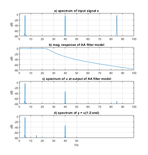
Figure 6.  5^th order, 0.1 dB Chebyshev anti-alias filter with sinusoidal inputs.  f_sadc = 100, R = 2.

a) Input spectrum of anti-alias filter.  b) Magnitude response of Anti-alias filter model.

c) Spectrum at output of anti-alias filter.  d) Spectrum at output of ADC.

Example 3.  Noise Aliasing

If you apply a signal with Gaussian noise directly to a wideband ADC, the noise above the Nyquist frequency creates aliases that raise the noise floor at the ADC output.  So even with no obvious signals at frequencies above f_sadc/2, aliasing may be important.  For our example we’ll model the Analog Devices AD9608 10-bit ADC, which has a maximum sample frequency of 125 MHz and bandwidth of 650 MHz [5].  We’ll let f_sadc = 125 MHz.  The input signal is a sinewave at 21 MHz with added Gaussian noise.  We’ll look at the output noise spectrum without and then with an anti-alias filter.

In the Matlab code below, we represent the ADC’s frequency response by using a 2^nd order Butterworth lowpass with f_c = 650 MHz.  We’ll use R = 16, giving filter model f_s = 16*125 MHz = 2000 MHz.  The function butter employs the bilinear transform to generate the coefficients, so the stopband is not that realistic.  However, exact stopband response is not critical when filtering noise, and using butter allows a lower sample rate in the model compared to a more realistic first order impulse-invariant filter.  For the spectrum calculations using psd_kaiser, we let nfft = N/8, where N is the number of time samples in the signal.  This is done to provide psd averaging, which smooths the Gaussian noise spectrum.

    fsadc= 125e6;                  % Hz ADC sample rate
    R= 16;                         % downsample ratio
    fs= R*fsadc;                   % Hz sample rate for ADC response model
    Ts= 1/fs;
    fc_adc= 650e6;                 % Hz adc analog bandwidth
    nbits= 10;                     % ADC number of bits
    f0= 21e6;                      % Hz sine frequency
    A= 0.5;                        % V sine amplitude (1 Vpp)
    [b_adc,a_adc]= butter(2,fc_adc/(fs/2));    % coeffs of adc response model
    N= 2^15;                        % number of samples
    n= 0:N-1;                       % sample index
    x= A*sin(2*pi*f0*n*Ts) + .015*randn(1,N);    % sine + noise
    u= filter(b_adc,a_adc,x);       % compute output of adc response model
    y= u(1:R:end);                  % downsample
    y= floor(y*2^nbits)/2^nbits;    % quantize (1 Vpp signal)
    % spectra of x, u, and y.Hz/bin = fs/(N/8)
    %[PdB1,f]= psd_kaiser(x,N/8,fs);        % spectrum of input signal
    [PdB2,f]= psd_kaiser(u,N/8,fs);         % spectrum at output of response model
    [PdB3,f2]= psd_kaiser(y,N/8/R,fs/R);    % spectrum at output of ADC

The Nyquist bandwidth of the ADC is f_sadc/2 = 62.5 MHz.  The ADC bandwidth of 650 MHz is approximately 10*f_sadc.  Sampling causes the noise in 9 Nyquist zones to alias to the first Nyquist zone and add to the noise in that frequency range.  We thus expect the output noise floor to rise by a factor of 10 or 10*log₁₀(10) = 10 dB relative to the analog signal’s noise floor.

Figure 7a shows the spectrum at the output of the ADC response model, with a -3 dB point at 650 MHz.  Figure 7b shows the ADC output spectrum (Both spectra have the same Hz/bin).  As expected, the ADC output’s noise floor is about 10 dB higher than the analog signal’s noise floor.  We see that wide ADC bandwidth can have an unintended bad effect on SNR.

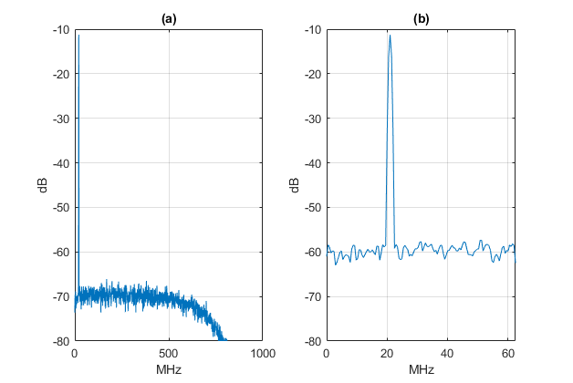
Figure 7.  Spectra of sine with added Gaussian noise, no anti-alias filter.

a) Spectrum at output of ADC response model, f_s = 2000 MHz.  488 kHz/bin.

b) Spectrum at output of ADC, f_sadc = 125 MHz.  488 kHz/bin.

A simple anti-alias filter can prevent the noise aliasing seen in Figure 7b.  The following code uses butter_impinvar to compute the coefficients of a 3^rd order Butterworth lowpass filter with f_c = 40 MHz.  The sample frequency f_s is the same as in the above code: f_s = R*f_sadc = 16*125 MHz = 2000 MHz.

    fc= 40e6;        % Hz AA filter cutoff freq
    order = 3;
    [b,a]= butter_impinvar(order,fc,fs);

The magnitude response of the filter is shown in Figure 8.  It has about 12 dB of attenuation at f_sadc/2 = 62.5 MHz.  Using this filter in place of the 650 MHz cutoff filter used above, the spectrum at the filter output is as shown in Figure 9a.  The spectrum at the ADC output is shown in Figure 9b, where we see that the noise floor has not increased from that of the input signal.  Again, both spectra have the same Hz/bin.

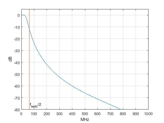
Figure 8.  Magnitude response of third-order analog Butterworth filter, f_c = 40 Hz.

            [h,f]= freqz(b,a,256,fs);
            HdB= 20*log10(abs(h));
            plot(f/1e6,HdB),grid,axis([0 fs/2e6 -80 5])

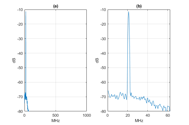
Figure 9.  Spectra of sine with added Gaussian noise, with f_c = 40 MHz anti-alias filter.

a) Spectrum at output of anti-alias filter, f_s = 2000 MHz.  488 kHz/bin.

b) Spectrum at output of ADC, f_sadc = 125 MHz.  488 kHz/bin.

For appendices, see the PDF version of this article.

References

1.  Kester, Walt, Ed., The Data Conversion Handbook, Elsevier, 2005, p. 76 – 77.

https://www.analog.com/en/education/education-library/data-conversion-handbook.html

2.  Lyons, Richard G., Understanding Digital Signal Processing, 3^rd Ed., sections 6.10 and 6.11.

3.  Blinchikoff, Herman J., and Zverev,Anatol I., Filtering in the Time and Frequency Domains, Wiley, 1976, section 3.4.1.

4.  Robertson, Neil, “Modeling a Continuous-Time System with Matlab”, DSPrelated.com, June, 2017, https://www.dsprelated.com/showarticle/1055.php

5.  AD9608 data sheet, Analog Devices, 2015, https://www.analog.com/en/products/ad9608.html?doc=AD9608.pdf

6.  Analog Devices Mini Tutorial MT-224, 2012, http://www.analog.com/media/en/training-seminars/tutorials/MT-224.pdf

7.  Blinchikoff and Zverev, section 3.4.2.

8.  Robertson, Neil, “A Simplified Matlab Function for Power Spectral Density”, DSPrelated.com, March, 2020, https://www.dsprelated.com/showarticle/1333.php

9.  RFtools website LC filter design tool, https://rf-tools.com/lc-filter/

10.  Coilcraft website, https://www.coilcraft.com/

Neil Robertson                    September, 2021

Sign in