Simple Discrete-Time Modeling of Lossy LC Filters

• Matlab

There are many software applications that allow modeling LC filters in the frequency domain.  But sometimes it is useful to have a time domain model, such as when you need to analyze a mixed analog and DSP system.  For example, the system in Figure 1 includes an LC filter as well as a DSP portion.  The LC filter could be an anti-alias filter, a channel filter, or some other LC network.  For a design using undersampling, the filter would be bandpass [1].  By modeling both the LC filter and DSP system in the time domain, we can analyze the whole system using one discrete-time model.  This approach inherently models the effects of nonlinear phase.  We can of course also obtain signal spectra by using the Discrete Fourier Transform (DFT)

In a previous post [2], I discussed modeling lowpass Butterworth or Chebyshev anti-alias filters using ideal IIR filter models.  This article employs a more general approach that allows modeling of arbitrary filter types (e.g., lowpass, bandpass), while also taking losses into account.  It does not matter how the LC filter is synthesized, whether by classical approximation (e.g., Butterworth) or by optimization.

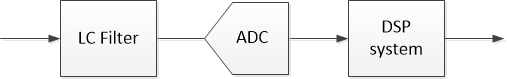
Figure 1.  Mixed Analog and DSP System.  (ADC:  Analog-to-Digital Converter)

Modeling Approach

The approach we’ll take is to find the frequency response of the LC filter, and then use the Inverse DFT (IDFT) to compute the impulse response.  Our model is then the impulse response, which can be viewed as an asymmetrical FIR filter.  This approach is simpler than some other methods, such as designing an IIR filter whose complex frequency response approximates that of the lossy LC filter [3], or using ODE (ordinary differential equation) integrator software like SPICE.

A summary of the steps to create the model is as follows:

1.  Create a filter schematic diagram, including resistive losses.

2.  Compute the discrete-frequency response G(k) using the chain matrix (ABCD parameters).

3.  Using G(k), create a frequency response H(k) with even-symmetric real part and odd-symmetric imaginary part.

4.  Compute the IDFT of H(k), which is the discrete-time impulse response h(n) of the filter.

We’ll try out the approach with an example LC filter, using a Matlab function to design the filter and find its impulse response.  Then we’ll examine how the Matlab function works.

Example – 5^th Order Butterworth LC lowpass filter

Figure 2 shows the schematic of a 5^th order LC lowpass filter with finite-Q inductors (The resistors R_series represent the loss of the inductors).  Using the Matlab function butterQdemo (Appendix A), we’ll synthesize a 5^th order LC Butterworth filter with a given cut-off frequency and find its discrete-time impulse response.  Appendix A also explains how to modify the Matlab function to model 5^th order Chebyshev filters.

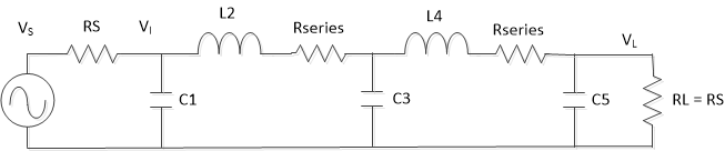
Figure 2.  LC Filter schematic diagram with lossy inductors.

Since capacitor Q is typically much higher than inductor Q, we’ll assume ideal capacitors for our model.  Inputs to the model include continuous-time and discrete-time parameters:  -3 dB frequency f_c, source resistance RS, inductor Q QL (evaluated at f = f_c), number of points in the impulse response N, and sample frequency f_s.  Here is the Matlab code to model a filter with f_c = 20 MHz, RS = 50 ohms, and QL = 30.  We’ll use f_s = 200 MHz and N = 128:

    fc= 20E6;             % Hz filter -3 dB frequency
    QL= 30;               %inductor Q at f = fc
    RS= 50;               % ohms source resistance
    N= 128;               % number of points in impulse/freq response
    fs= 200E6;            % Hz sample frequency
    [H,f,h]= butterQdemo(fc,QL,RS,N,fs);
    HdB= 20*log10(abs(H));    % dB magnitude response

The outputs of butterQdemo are the discrete-frequency response H(k) and a corresponding frequency vector f of N points over 0 to fs; and the discrete-time impulse response h(n) of length N.  The function also prints the capacitor and inductor values and the value of R_series.  For our example, these values are:

C1 = 98.4 pF, C3 = 31.8 pF, C5 = 98.4 pF

L2 = 644 nH, L4 = 644 nH

Rseries = 2.70 ohms

The frequency response dB magnitude is plotted in Figure 3, along with the response of an ideal filter.  Insertion loss of the lossy filter at 20 MHz is about 3.8 dB, compared to 3.01 dB for the ideal filter. The impulse response h(n) is plotted in Figure 4, along with the impulse response of an ideal filter (Note we have plotted only the first 50 samples).  h(n) is the discrete-time filter model that we set out to find. 

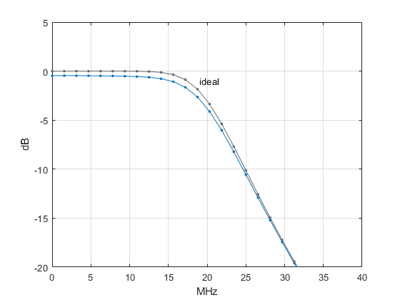
Figure 3.  5^th order Butterworth filter model dB Magnitude response, f_c = 20 MHz, QL = 30, f_s = 200 MHz.

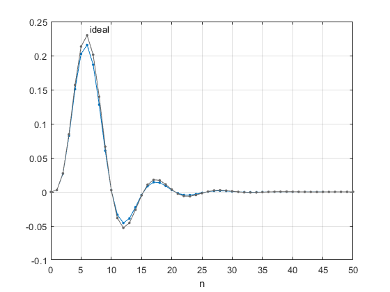
Figure 4.  5^th order Butterworth filter model impulse response h(n), QL = 30 at f_c.

How it Works

The Matlab function butterQdemo is listed in Appendix A.  This simple function only allows for 5^th order lowpass filters.  A more general approach would be to start out with the schematic of an LC filter designed using filter synthesis software.  For example, a free online synthesis tool is available at the RF Tools website [4].

As mentioned, the model inputs include -3 dB frequency f_c, source resistance RS, and inductor Q QL. The function starts with normalized L and C values computed for RS = RL = 1 ohm and ω_c = 2πf_c = 1 rad/s.  These values are then scaled according to:

$$ C = \frac{C_{norm}}{2\pi f_c R_s} \qquad (1) $$

$$ L = \frac{L_{norm}R_s}{2\pi f_c} \qquad (2) $$

Scaling results in a filter that has the desired f_c when terminated with source resistance RS and load resistance RL = RS.  The filter schematic diagram is repeated in Figure 5 (top).  After component value scaling, the value of inductor loss R_series is calculated.  For simplicity, we assume R_series is constant vs. frequency.  Defining Q at ω = ω_c, inductor Q is given by:

$$ QL= \frac{\omega_c L}{R_{series}} \qquad (3) $$

Thus,

$$ R_{series}= \frac{2\pi f_c L}{QL} \qquad (4) $$

Next, the filter’s branches are converted to series impedance (Z) elements and shunt admittance (Y) elements for chain matrix analysis, as shown in Figure 5 (bottom).  The chain matrix is discussed in Appendix B.  The capacitors are assumed ideal and their Y values are:

$$ Y = j\omega C + 1/R_{shunt} \approx j\omega C \qquad (5) $$

Where ω is a vector of radian frequencies:

$$ \omega = \frac{2\pi k f_s}{N},\; k= 0: N/2 \qquad (6) $$

and N is the number of frequency samples from 0 to f_s.  The lossy-inductor Z values are:

$$ Z= j\omega L + R_{series} \qquad (7) $$

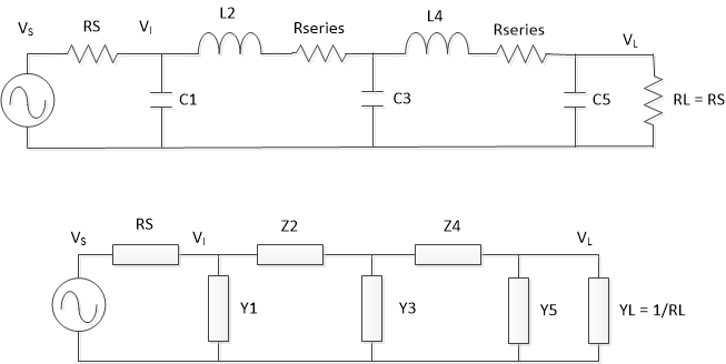
Figure 5.  Filter from Example 1.  Top:  Schematic Diagram.

Bottom:  Filter series-Z and shunt-Y elements for chain matrix.

Once all the Z and Y elements have been computed, the chain matrix is evaluated to determine the frequency response G(k).  For a continuous-time system, G(ω) extends to infinite frequency, while for our discrete-time model, we have defined G(k) up to the Nyquist frequency, f = f_s/2 (k = N/2).  G(k) is complex, as shown in Figure 6 for our example filter.  The magnitude response is shown in the bottom plot of Figure 6 with a linear amplitude scale.

We now want to use G(k) and the IDFT to find a real-valued impulse response.  But we cannot use G(k) as is, because it does not meet a key property of the DFT – namely, for a real h(n), the DFT H(k) has real part even-symmetric with respect to N/2 and imaginary part odd-symmetric.  Since we require h(n) to be real, we need to create an H(k) with this property from our G(k).  This can is done using the following equations, where we note that the index of G has a range of k = 0: N/2:

$$ G_c(k)= conj(G(1:N/2-1)) \qquad (8) $$

$$ H(k)= [G \; flip(G_c)] \qquad (9) $$

Where conj( ) is the complex conjugate and flip reverses the order of G_c.  H has length N.  Matlab does not allow a zero index, so these equations translate to the Matlab code:

    Gc = conj(G(2:N/2));     % complex conjugate of G
    H = [G fliplr(Gc)];

This gives us the frequency response H(k) shown in Figure 7, where, as desired, the real part is even-symmetric with respect to N/2 and the imaginary part is odd-symmetric.  The magnitude response is shown at the bottom with a linear amplitude scale.  The final step is to take the IDFT of H(k), giving real h(n) with length N.

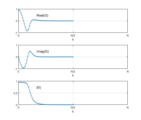
Figure 6.  Frequency Response G(k) of LC Filter from circuit model, f_c = f_s/10, QL = 30 at f = f_c.  Top:  Real part.  Middle:  Imaginary part.  Bottom:  Magnitude.

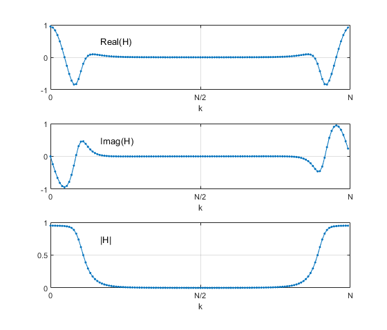
Figure 7.  Frequency Response H(k) with even symmetric real part and odd-symmetric imaginary part, f_c = f_s/10, QL = 30 at f = f_c.  Top:  Real part.  Middle:  Imaginary part.  Bottom:  Magnitude.

Requirements on Model Parameters

The model is not overly sensitive to its input parameters, but it is possible to go astray.  Here are two requirements to achieve accurate results:

1.  Sample rate f_s must be sufficiently high relative to f_c.  Suppose we want to model a filter with stopband of -50 dB.  Then the filter’s magnitude response at the Nyquist frequency |H(f_s/2)| must be less than -50 dB.  If this is not the case, f_s must be increased so that the required attenuation is exceeded at f_s/2.
2.  N must be sufficiently large.  Since N is the number of samples in h(n), N must be large enough to allow h(n) to settle.  Conversely, if h(n) is sufficiently small at some n < N, it may be truncated to reduce the total number of samples.  Looking at this issue from a frequency domain perspective:  our chain matrix frequency response H(k) is a sampled version of the continuous frequency response H(f).  The DFT of h(n) is guaranteed to match H(f) only at the N sample frequencies.  If we were to zero-pad h(n) and then take the DFT, we would create new frequency samples at a finer spacing.  These new frequency samples would deviate from H(f) to some degree.  Larger values of N reduce this deviation.

Sanity Checks

As a check on our approach, we can compare our model’s h(n) for an ideal lowpass to that of a 5^th order Butterworth IIR filter designed using the impulse invariance method [2].  The two impulse responses are plotted in Figure 8, and the (small) error of the IDFT impulse response with respect to the IIR impulse response is plotted in Figure 9.

It is not always necessary to retain all N points of h(n).  As an example, our original example used N = 128.Suppose we truncate h(n) to 64 points and compute its 128-point DFT:

    H2= fft(h(1:64),N);
    H2dB= 20*log10(abs(H2));

Figure 10 plots H2dB along with the original magnitude response.  The error of H2dB does not reach 1 dB until HdB = -67 dB.

Finally, as already mentioned, the DFT of h(n) is guaranteed to match H(f) only at the N sample frequencies.  If we zero-pad h(n) and then take the DFT, the new frequency points will deviate from H(f) to some degree.  Figure 11 plots the dB magnitude response of our original example filter, along with the response of the DFT of a zero-padded h(n).  The responses track well for attenuations up to roughly 60 dB.

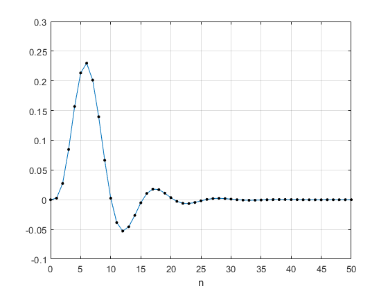
Figure 8.  Ideal 5^th order Butterworth impulse response using two methods, f_c = f_s/10.

Solid line:  IDFT method.  Dots:  Impulse-invariance method.

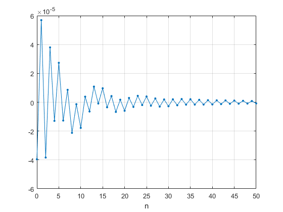
Figure 9.  Impulse response absolute error of IDFT method vs. Impulse-invariance method.

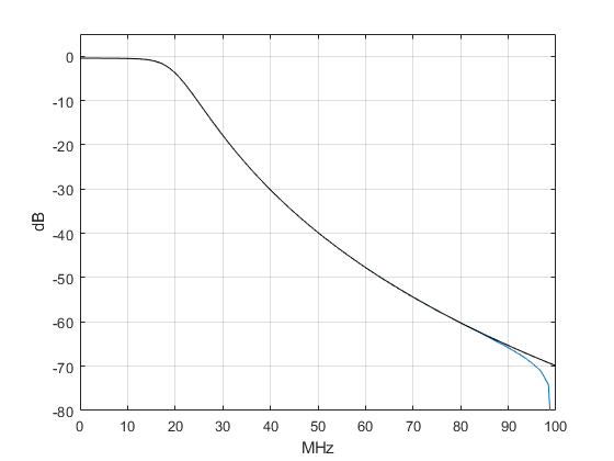
Figure 10.  Effect on magnitude response of truncating h(n).  5^th order Butterworth filter, f_c= 20 MHz, QL= 30, f_s= 200 MHz.  Black:  Chain matrix response, N= 128.  Blue:  Magnitude of fft(h(1:64),N).

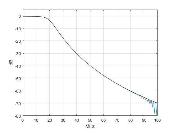
Figure 11.  Effect on magnitude response of zero-padding h(n).  5^th order Butterworth filter, f_c= 20 MHz, QL= 30, f_s= 200 MHz.  Black:  Chain matrix response, N= 128. Blue:  DFT of zero-padded h(n), N= 1024.

Modeling Bandpass and Highpass LC Filters

The approach used here works well for bandpass filters, as long as the filter’s upper stopband has sufficient attenuation at f = f_s/2.  As already mentioned, a filter can be designed using web-based filter synthesis software [4].  Component losses can then be added to the filter schematic, and the filter modeled as already described.

Our modeling approach does not work well for pure high-pass filters, because the imaginary part of H(k) is typically not small at the Nyquist frequency.  This causes a discontinuity in H(k) at k = N/2 and an error in h(n).  However, any mixed-signal system contains a lowpass or bandpass analog filter, either as an anti-alias filter or DAC reconstruction filter.  So, a highpass filter can be modeled by cascading it with one of these filters.

See the PDF version of this article for Appendices.

References

1.  Kester, Walt, Ed., Data Conversion Handbook, Newnes, 2005, p 80 - 81.   https://www.analog.com/en/education/education-library/data-conversion-handbook.html
2.  Robertson, Neil, “Modeling Anti-alias Filters,” DSPrelated.com, Sept, 2021, https://www.dsprelated.com/showarticle/1418.php
3.  Lyons, Richard G., Understanding Digital Signal Processing, 3^rd Ed., Pearson, 2011, p 330 – 331.
4.  RFTools.com, “LC Filter Design Tool,” Marki Microwave,https://rf-tools.com/lc-filter/
5.  Williams, Arthur B., Electronic Filter Design Handbook, 3^rd Ed., McGraw Hill, 1995, p 2.35.
6.  Williams, p 11.28.
7.  Ludwig, Reinhold and Bogdanov, Gene, RF Circuit Design, 2^nd Ed., Pearson, 2009, p 163.

Neil Robertson           April, 2023

Sign in