


State Space Models
Equations of motion for any physical system may be conveniently formulated in terms of the state of the system [330]:
Here,
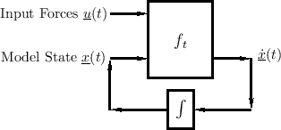
Equation (1.6) is diagrammed in Fig.1.4.
The key property of the state vector
![]() in this formulation is
that it completely determines the system at time
in this formulation is
that it completely determines the system at time ![]() , so that
future states depend only on the current state and on any inputs at
time
, so that
future states depend only on the current state and on any inputs at
time ![]() and beyond.2.8 In particular, all past states and the
entire input history are ``summarized'' by the current state
and beyond.2.8 In particular, all past states and the
entire input history are ``summarized'' by the current state
![]() .
Thus,
.
Thus,
![]() must include all ``memory'' of the system.
must include all ``memory'' of the system.
Forming Outputs
Any system output is some function of the state, and possibly the input (directly):
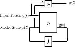
The general case of output extraction is shown in Fig.1.5.
The output signal (vector) is most typically a linear combination of state variables and possibly the current input:
State-Space Model of a Force-Driven Mass
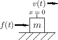
For the simple example of a mass ![]() driven by external force
driven by external force ![]() along the
along the ![]() axis, we have the system of Fig.1.6.
We should choose the state variable to be velocity
axis, we have the system of Fig.1.6.
We should choose the state variable to be velocity
![]() so that
Newton's
so that
Newton's ![]() yields
yields
Numerical Integration of General State-Space Models
An approximate discrete-time numerical solution of Eq.![]() (1.6) is provided by
(1.6) is provided by
Let
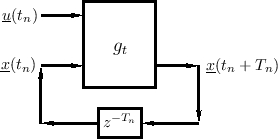
This is a simple example of numerical integration for solving
an ODE, where in this case the ODE is given by Eq.![]() (1.6) (a very
general, potentially nonlinear, vector ODE). Note that the initial
state
(1.6) (a very
general, potentially nonlinear, vector ODE). Note that the initial
state
![]() is required to start Eq.
is required to start Eq.![]() (1.7) at time zero;
the initial state thus provides boundary conditions for the ODE at
time zero. The time sampling interval
(1.7) at time zero;
the initial state thus provides boundary conditions for the ODE at
time zero. The time sampling interval ![]() may be fixed for all
time as
may be fixed for all
time as ![]() (as it normally is in linear, time-invariant
digital signal processing systems), or it may vary adaptively
according to how fast the system is changing (as is often needed for
nonlinear and/or time-varying systems). Further discussion of
nonlinear ODE solvers is taken up in §7.4, but for most of
this book, linear, time-invariant systems will be emphasized.
(as it normally is in linear, time-invariant
digital signal processing systems), or it may vary adaptively
according to how fast the system is changing (as is often needed for
nonlinear and/or time-varying systems). Further discussion of
nonlinear ODE solvers is taken up in §7.4, but for most of
this book, linear, time-invariant systems will be emphasized.
Note that for handling switching states (such as op-amp
comparators and the like), the discrete-time state-space formulation
of Eq.![]() (1.7) is more conveniently applicable than the
continuous-time formulation in Eq.
(1.7) is more conveniently applicable than the
continuous-time formulation in Eq.![]() (1.6).
(1.6).
State Definition
In view of the above discussion, it is perhaps plausible that the
state
![]() of a physical
system at time
of a physical
system at time ![]() can be defined as a collection of state
variables
can be defined as a collection of state
variables ![]() , wherein each state variable
, wherein each state variable ![]() is a
physical amplitude (pressure, velocity, position,
is a
physical amplitude (pressure, velocity, position, ![]() )
corresponding to a degree of freedom of the system. We define a
degree of freedom as a single dimension of energy
storage. The net result is that it is possible to compute the
stored energy in any degree of freedom (the system's ``memory'') from
its corresponding state-variable amplitude.
)
corresponding to a degree of freedom of the system. We define a
degree of freedom as a single dimension of energy
storage. The net result is that it is possible to compute the
stored energy in any degree of freedom (the system's ``memory'') from
its corresponding state-variable amplitude.
For example, an ideal mass ![]() can store only kinetic
energy
can store only kinetic
energy
![]() , where
, where
![]() denotes the
mass's velocity along the
denotes the
mass's velocity along the ![]() axis. Therefore, velocity is the
natural choice of state variable for an ideal point-mass.
Coincidentally, we reached this conclusion independently above by
writing
axis. Therefore, velocity is the
natural choice of state variable for an ideal point-mass.
Coincidentally, we reached this conclusion independently above by
writing ![]() in state-space form
in state-space form
![]() . Note that a
point mass that can move freely in 3D space has three degrees of
freedom and therefore needs three state variables
. Note that a
point mass that can move freely in 3D space has three degrees of
freedom and therefore needs three state variables
![]() in
its physical model. In typical models from musical acoustics (e.g.,
for the piano hammer), masses are allowed only one degree of freedom,
corresponding to being constrained to move along a 1D line, like an
ideal spring. We'll study the ideal mass further in §7.1.2.
in
its physical model. In typical models from musical acoustics (e.g.,
for the piano hammer), masses are allowed only one degree of freedom,
corresponding to being constrained to move along a 1D line, like an
ideal spring. We'll study the ideal mass further in §7.1.2.
Another state-variable example is provided by an ideal spring
described by Hooke's law ![]() (§B.1.3), where
(§B.1.3), where ![]() denotes the spring
constant, and
denotes the spring
constant, and ![]() denotes the spring displacement from rest. Springs
thus contribute a force proportional to displacement in Newtonian
ODEs. Such a spring can only store the physical work (force
times distance), expended to displace, it in the form of
potential energy
denotes the spring displacement from rest. Springs
thus contribute a force proportional to displacement in Newtonian
ODEs. Such a spring can only store the physical work (force
times distance), expended to displace, it in the form of
potential energy
![]() . More about
ideal springs will be discussed in §7.1.3. Thus,
spring displacement is the most natural choice of state
variable for a spring.
. More about
ideal springs will be discussed in §7.1.3. Thus,
spring displacement is the most natural choice of state
variable for a spring.
In so-called RLC electrical circuits (consisting of resistors ![]() ,
inductors
,
inductors ![]() , and capacitors
, and capacitors ![]() ), the state variables are
typically defined as all of the capacitor voltages (or charges) and
inductor currents. We will discuss RLC electrical circuits further
below.
), the state variables are
typically defined as all of the capacitor voltages (or charges) and
inductor currents. We will discuss RLC electrical circuits further
below.
There is no state variable for each resistor current in an RLC circuit
because a resistor dissipates energy but does not store it--it has no
``memory'' like capacitors and inductors. The state (current ![]() ,
say) of a resistor
,
say) of a resistor ![]() is determined by the voltage
is determined by the voltage ![]() across it,
according to Ohm's law
across it,
according to Ohm's law ![]() , and that voltage is supplied by the
capacitors, inductors, and voltage-sources, etc., to which it is
connected. Analogous remarks apply to the dashpot, which is
the mechanical analog of the resistor--we do not assign state
variables to dashpots. (If we do, such as by mistake, then we will
obtain state variables that are linearly dependent on other state
variables, and the order of the system appears to be larger than it
really is. This does not normally cause problems, and there are many
numerical ways to later ``prune'' the state down to its proper order.)
, and that voltage is supplied by the
capacitors, inductors, and voltage-sources, etc., to which it is
connected. Analogous remarks apply to the dashpot, which is
the mechanical analog of the resistor--we do not assign state
variables to dashpots. (If we do, such as by mistake, then we will
obtain state variables that are linearly dependent on other state
variables, and the order of the system appears to be larger than it
really is. This does not normally cause problems, and there are many
numerical ways to later ``prune'' the state down to its proper order.)
Masses, springs, dashpots, inductors, capacitors, and resistors are examples of so-called lumped elements. Perhaps the simplest distributed element is the continuous ideal delay line. Because it carries a continuum of independent amplitudes, the order (number of state variables) is infinity for a continuous delay line of any length! However, in practice, we often work with sampled, bandlimited systems, and in this domain, delay lines have a finite number of state variables (one for each delay element). Networks of lumped elements yield finite-order state-space models, while even one distributed element jumps the order to infinity until it is bandlimited and sampled.
In summary, a state variable may be defined as a physical amplitude for some energy-storing degree of freedom. In models of mechanical systems, a state variable is needed for each ideal spring and point mass (times the number of dimensions in which it can move). For RLC electric circuits, a state variable is needed for each capacitor and inductor. If there are any switches, their state is also needed in the state vector (e.g., as boolean variables). In discrete-time systems such as digital filters, each unit-sample delay element contributes one (continuous) state variable to the model.
Next Section:
Linear State Space Models
Previous Section:
Difference Equations (Finite Difference Schemes)


