


Background Fundamentals
Signal Representation and Notation
Below is a summary of various notational conventions used in digital signal processing for representing signals and spectra. For a more detailed presentation, see the elementary introduction to signal representation, sinusoids, and exponentials in [84].A.1
Units
In this book, time ![]() is always in physical units of seconds
(s), while time
is always in physical units of seconds
(s), while time ![]() or
or ![]() is in units of samples (counting
numbers having no physical units). Time
is in units of samples (counting
numbers having no physical units). Time ![]() is a continuous real
variable, while discrete-time in samples is integer-valued. The
physical time
is a continuous real
variable, while discrete-time in samples is integer-valued. The
physical time ![]() corresponding to time
corresponding to time ![]() in samples is given by
in samples is given by
For frequencies, we have two physical units: (1)
cycles per second and (2) radians per second. The
name for cycles per second is Hertz (Hz) (though in the past it
was cps). One cycle equals ![]() radians, which is 360
degrees (
radians, which is 360
degrees (![]() ). Therefore,
). Therefore, ![]() Hz is the same frequency as
Hz is the same frequency as ![]() radians per second (rad/s). It is easy to confuse the two because
both radians and cycles are pure numbers, so that both types of
frequency are in physical units of inverse seconds (s
radians per second (rad/s). It is easy to confuse the two because
both radians and cycles are pure numbers, so that both types of
frequency are in physical units of inverse seconds (s
![]() ).
).
For example, a periodic signal with a period of ![]() seconds has
a frequency of
seconds has
a frequency of ![]() Hz, and a radian frequency of
Hz, and a radian frequency of
![]() rad/s. The sampling rate,
rad/s. The sampling rate, ![]() , is the reciprocal of the
sampling period
, is the reciprocal of the
sampling period ![]() , i.e.,
, i.e.,
Sinusoids
The term sinusoid means a waveform of the type
Thus, a sinusoid may be defined as a cosine at amplitude
![$\displaystyle f(t) \isdef \frac{d}{dt} \theta(t) = \frac{d}{dt} \left[\omega t + \phi\right] = \omega
$](http://www.dsprelated.com/josimages_new/filters/img1302.png)
Spectrum
In this book, we think of filters primarily in terms of their effect
on the spectrum of a signal. This is appropriate because the
ear (to a first approximation) converts the time-waveform at the
eardrum into a neurologically encoded spectrum. Intuitively, a
spectrum (a complex function of frequency ![]() ) gives the
amplitude and phase of the sinusoidal signal-component at frequency
) gives the
amplitude and phase of the sinusoidal signal-component at frequency
![]() . Mathematically, the spectrum of a signal
. Mathematically, the spectrum of a signal ![]() is the Fourier
transform of its time-waveform. Equivalently, the spectrum is the
z transform evaluated on the unit circle
is the Fourier
transform of its time-waveform. Equivalently, the spectrum is the
z transform evaluated on the unit circle
![]() . A detailed
introduction to spectrum analysis is given in
[84].A.2
. A detailed
introduction to spectrum analysis is given in
[84].A.2
We denote both the spectrum and the z transform of a signal by uppercase
letters. For example, if the time-waveform is denoted ![]() , its z transform
is called
, its z transform
is called ![]() and its spectrum is therefore
and its spectrum is therefore
![]() . The
time-waveform
. The
time-waveform ![]() is said to ``correspond'' to its z transform
is said to ``correspond'' to its z transform ![]() ,
meaning they are transform pairs. This correspondence is often denoted
,
meaning they are transform pairs. This correspondence is often denoted
![]() , or
, or
![]() . Both
the z transform and its special case, the (discrete-time) Fourier transform,
are said to transform from the time domain to the
frequency domain.
. Both
the z transform and its special case, the (discrete-time) Fourier transform,
are said to transform from the time domain to the
frequency domain.
We deal most often with discrete time ![]() (or simply
(or simply ![]() ) but
continuous frequency
) but
continuous frequency ![]() (or
(or
![]() ). This is because the
computer can represent only digital signals, and digital
time-waveforms are discrete in time but may have energy at any
frequency. On the other hand, if we were going to talk about FFTs
(Fast Fourier Transforms--efficient implementations of the Discrete
Fourier Transform, or DFT) [84], then we would have to
discretize the frequency variable also in order to represent spectra
inside the computer. In this book, however, we use spectra only for
conceptual insights into the perceptual effects of digital filtering;
therefore, we avoid discrete frequency for simplicity.
). This is because the
computer can represent only digital signals, and digital
time-waveforms are discrete in time but may have energy at any
frequency. On the other hand, if we were going to talk about FFTs
(Fast Fourier Transforms--efficient implementations of the Discrete
Fourier Transform, or DFT) [84], then we would have to
discretize the frequency variable also in order to represent spectra
inside the computer. In this book, however, we use spectra only for
conceptual insights into the perceptual effects of digital filtering;
therefore, we avoid discrete frequency for simplicity.
When we wish to consider an entire signal as a ``thing in itself,'' we
write ![]() , meaning the whole time-waveform (
, meaning the whole time-waveform (![]() for all
for all
![]() ), or
), or ![]() , to mean the entire spectrum taken as a whole.
Imagine, for example, that we have plotted
, to mean the entire spectrum taken as a whole.
Imagine, for example, that we have plotted ![]() on a strip of paper
that is infinitely long. Then
on a strip of paper
that is infinitely long. Then ![]() refers to the complete
picture, while
refers to the complete
picture, while ![]() refers to the
refers to the ![]() th sample point on the plot.
th sample point on the plot.
Complex and Trigonometric Identities
This section gives a summary of some of the more useful mathematical identities for complex numbers and trigonometry in the context of digital filter analysis. For many more, see handbooks of mathematical functions such as Abramowitz and Stegun [2].
The symbol ![]() means ``is defined as'';
means ``is defined as''; ![]() stands for a complex
number; and
stands for a complex
number; and ![]() ,
, ![]() ,
, ![]() , and
, and ![]() stand for real numbers. The
quantity
stand for real numbers. The
quantity ![]() is used below to denote
is used below to denote
![]() .
.
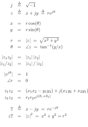
Complex Numbers
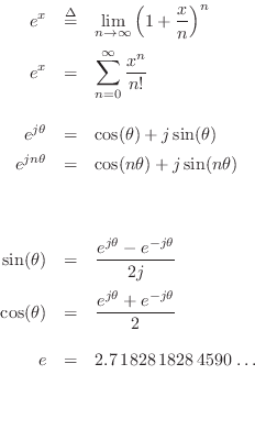
The Exponential Function
Trigonometric Identities
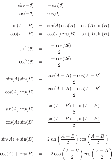
Trigonometric Identities, Continued

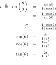
Half-Angle Tangent Identities
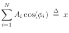
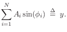
A Sum of Sinusoids at the
Same Frequency is Another
Sinusoid at that Frequency
It is an important and fundamental fact that a sum of sinusoids at the same frequency, but different phase and amplitude, can always be expressed as a single sinusoid at that frequency with some resultant phase and amplitude. An important implication, for example, is that
That is, if a sinusoid is input to an LTI system, the output will be a sinusoid at the same frequency, but possibly altered in amplitude and phase. This follows because the output of every LTI system can be expressed as a linear combination of delayed copies of the input signal. In this section, we derive this important result for the general case of
Proof Using Trigonometry
We want to show it is always possible to solve
for
| (A.3) |
Applying this expansion to Eq.
![\begin{eqnarray*}
\left[A\cos(\phi)\right]\cos(\omega t)
&-&\left[A\sin(\phi)\ri...
...a t)
- \left[\sum_{i=1}^N A_i\sin(\phi_i)\right]\sin(\omega t).
\end{eqnarray*}](http://www.dsprelated.com/josimages_new/filters/img1320.png)
Equating coefficients gives
where

which has a unique solution for any values of ![]() and
and ![]() .
.
Proof Using Complex Variables
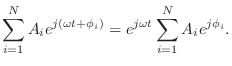
To show by means of phasor analysis that Eq.![]() (A.2) always has a solution, we can express each component sinusoid as
(A.2) always has a solution, we can express each component sinusoid as
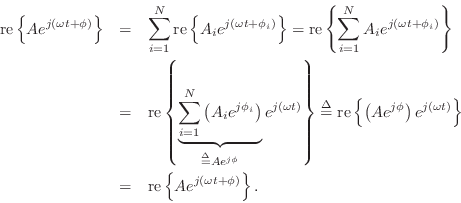
Thus, equality holds when we define
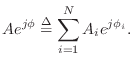
Since
As is often the case, we see that the use of Euler's identity and complex analysis gives a simplified algebraic proof which replaces a proof based on trigonometric identities.
Phasor Analysis: Factoring a Complex Sinusoid into Phasor Times Carrier
The heart of the preceding proof was the algebraic manipulation
For an arbitrary sinusoid having amplitude ![]() , phase
, phase ![]() , and
radian frequency
, and
radian frequency ![]() , we have
, we have
Next Section:
Elementary Audio Digital Filters
Previous Section:
Conclusion


