


Digitizing Analog Filters with the
Bilinear Transformation
The desirable properties of many filter types (such as lowpass,
highpass, and bandpass) are preserved very well by the
![]() mapping called the bilinear transform.
mapping called the bilinear transform.
Bilinear Transformation
The bilinear transform may be defined by


where
Frequency Warping
It is easy to check that the bilinear transform gives a one-to-one,
order-preserving, conformal map [57] between the
analog frequency axis
![]() and the digital frequency axis
and the digital frequency axis
![]() , where
, where ![]() is the sampling interval. Therefore, the
amplitude response takes on exactly the same values over both axes,
with the only defect being a
frequency warping such
that equal increments along the unit circle in the
is the sampling interval. Therefore, the
amplitude response takes on exactly the same values over both axes,
with the only defect being a
frequency warping such
that equal increments along the unit circle in the ![]() plane
correspond to larger and larger bandwidths along the
plane
correspond to larger and larger bandwidths along the ![]() axis in
the
axis in
the ![]() plane [88]. Some kind of frequency warping
is obviously unavoidable in any one-to-one map because the analog
frequency axis is infinite while the digital frequency axis is finite.
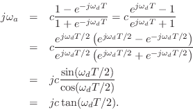
The relation between the analog and digital frequency axes may be
derived immediately from Eq.
plane [88]. Some kind of frequency warping
is obviously unavoidable in any one-to-one map because the analog
frequency axis is infinite while the digital frequency axis is finite.
The relation between the analog and digital frequency axes may be
derived immediately from Eq.![]() (I.9) as
(I.9) as
Given an analog cut-off frequency
![]() , to obtain the
same cut-off frequency in the digital filter, we set
, to obtain the
same cut-off frequency in the digital filter, we set
Analog Prototype Filter
Since the digital cut-off frequency may be set to any value,
irrespective of the analog cut-off frequency, it is convenient to set
the analog cut-off frequency to
![]() . In this case, the
bilinear-transform constant
. In this case, the
bilinear-transform constant ![]() is simply set to
is simply set to
Examples
Examples of using the bilinear transform to ``digitize'' analog filters may be found in §I.2 and [64,5,6,103,86]. Bilinear transform design is also inherent in the construction of wave digital filters [25,86].
Next Section:
Filter Design by Minimizing the L2 Equation-Error Norm
Previous Section:
Butterworth Lowpass Design


