


Butterworth Lowpass Design
Almost all methods for filter design are optimal in some sense,
and the choice of optimality determines nature of the design.
Butterworth filters are optimal in the sense of having a
maximally flat amplitude response, as measured using a Taylor
series expansion about dc [64, p. 162]. Of course,
the trivial filter ![]() has a perfectly flat amplitude response,
but that's an allpass, not a lowpass filter. Therefore, to constrain the
optimization to the space of lowpass filters, we need
constraints on the design, such as
has a perfectly flat amplitude response,
but that's an allpass, not a lowpass filter. Therefore, to constrain the
optimization to the space of lowpass filters, we need
constraints on the design, such as ![]() and
and ![]() .
That is, we may require the dc gain to be 1, and the gain at half the
sampling rate to be 0.
.
That is, we may require the dc gain to be 1, and the gain at half the
sampling rate to be 0.
It turns out Butterworth filters (as well as Chebyshev and Elliptic
Function filter types) are much easier to design as analog
filters which are then converted to digital filters. This means
carrying out the design over the ![]() plane instead of the
plane instead of the ![]() plane,
where the
plane,
where the ![]() plane is the complex plane over which analog filter
transfer functions are defined. The analog transfer function
plane is the complex plane over which analog filter
transfer functions are defined. The analog transfer function ![]() is very much like the digital transfer function
is very much like the digital transfer function ![]() , except that it
is interpreted relative to the analog frequency axis
, except that it
is interpreted relative to the analog frequency axis
![]() (the ``
(the ``![]() axis'') instead of the digital frequency axis
axis'') instead of the digital frequency axis
![]() (the ``unit circle''). In particular, analog filter poles
are stable if and only if they are all in the left-half of the
(the ``unit circle''). In particular, analog filter poles
are stable if and only if they are all in the left-half of the
![]() plane, i.e., their real parts are negative. An
introduction to Laplace transforms is given in Appendix D, and an
introduction to converting analog transfer functions to digital
transfer functions using the bilinear transform appears in
§I.3.
plane, i.e., their real parts are negative. An
introduction to Laplace transforms is given in Appendix D, and an
introduction to converting analog transfer functions to digital
transfer functions using the bilinear transform appears in
§I.3.
Butterworth Lowpass Poles and Zeros
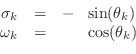
When the maximally flat optimality criterion is applied to the general
(analog) squared amplitude response
![]() , a surprisingly simple
result is obtained [64]:
, a surprisingly simple
result is obtained [64]:
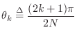
where
The analytic continuation
(§D.2)
of
![]() to the whole
to the whole
![]() -plane may be obtained by substituting
-plane may be obtained by substituting
![]() to obtain
to obtain

with
A Butterworth lowpass filter additionally has ![]() zeros at
zeros at ![]() .
Under the bilinear transform
.
Under the bilinear transform
![]() , these all map to the
point
, these all map to the
point ![]() , which determines the numerator of the digital filter as
, which determines the numerator of the digital filter as
![]() .
.
Given the poles and zeros of the analog prototype, it is straightforward to convert to digital form by means of the bilinear transformation.
Example: Second-Order Butterworth Lowpass
In the second-order case, we have, for the analog prototype,
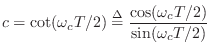
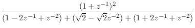
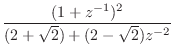
To convert this to digital form, we apply the bilinear transform

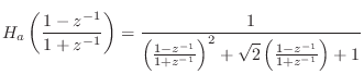 |
(I.4) | ||
 |
(I.5) | ||
 |
(I.6) | ||
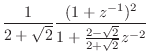 |
(I.7) |
Note that the numerator is

In the analog prototype,
the cut-off frequency is
![]() rad/sec, where,
from Eq.
rad/sec, where,
from Eq.![]() (I.1), the amplitude response
is
(I.1), the amplitude response
is
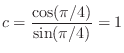
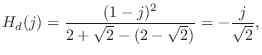
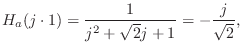
![]() . Since we mapped the cut-off frequency precisely
under the bilinear transform, we expect the digital filter to have
precisely this gain.
The digital frequency response at one-fourth the sampling rate is
. Since we mapped the cut-off frequency precisely
under the bilinear transform, we expect the digital filter to have
precisely this gain.
The digital frequency response at one-fourth the sampling rate is
and
Note from Eq.![]() (I.8) that the phase at cut-off is exactly -90 degrees
in the digital filter. This can be verified against the pole-zero
diagram in the
(I.8) that the phase at cut-off is exactly -90 degrees
in the digital filter. This can be verified against the pole-zero
diagram in the ![]() plane, which has two zeros at
plane, which has two zeros at ![]() , each
contributing +45 degrees, and two poles at
, each
contributing +45 degrees, and two poles at
![]() , each contributing -90
degrees. Thus, the calculated phase-response at the cut-off frequency
agrees with what we expect from the digital pole-zero diagram.
, each contributing -90
degrees. Thus, the calculated phase-response at the cut-off frequency
agrees with what we expect from the digital pole-zero diagram.
In the ![]() plane, it is not as easy to use the pole-zero diagram
to calculate the phase at
plane, it is not as easy to use the pole-zero diagram
to calculate the phase at
![]() , but using Eq.
, but using Eq.![]() (I.3), we
quickly obtain
(I.3), we
quickly obtain
A related example appears in §9.2.4.
Next Section:
Digitizing Analog Filters with the Bilinear Transformation
Previous Section:
Lowpass Filter Design


