


Example: Second-Order Butterworth Lowpass
In the second-order case, we have, for the analog prototype,
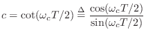
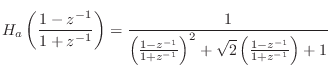
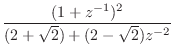
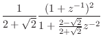
To convert this to digital form, we apply the bilinear transform

 |
(I.4) | ||
 |
(I.5) | ||
 |
(I.6) | ||
 |
(I.7) |
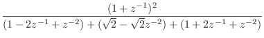
Note that the numerator is

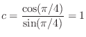
In the analog prototype,
the cut-off frequency is
![]() rad/sec, where,
from Eq.
rad/sec, where,
from Eq.![]() (I.1), the amplitude response
is
(I.1), the amplitude response
is
![]() . Since we mapped the cut-off frequency precisely
under the bilinear transform, we expect the digital filter to have
precisely this gain.
The digital frequency response at one-fourth the sampling rate is
. Since we mapped the cut-off frequency precisely
under the bilinear transform, we expect the digital filter to have
precisely this gain.
The digital frequency response at one-fourth the sampling rate is
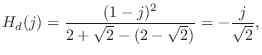
and
Note from Eq.![]() (I.8) that the phase at cut-off is exactly -90 degrees
in the digital filter. This can be verified against the pole-zero
diagram in the
(I.8) that the phase at cut-off is exactly -90 degrees
in the digital filter. This can be verified against the pole-zero
diagram in the ![]() plane, which has two zeros at
plane, which has two zeros at ![]() , each
contributing +45 degrees, and two poles at
, each
contributing +45 degrees, and two poles at
![]() , each contributing -90
degrees. Thus, the calculated phase-response at the cut-off frequency
agrees with what we expect from the digital pole-zero diagram.
, each contributing -90
degrees. Thus, the calculated phase-response at the cut-off frequency
agrees with what we expect from the digital pole-zero diagram.
In the ![]() plane, it is not as easy to use the pole-zero diagram
to calculate the phase at
plane, it is not as easy to use the pole-zero diagram
to calculate the phase at
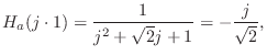
![]() , but using Eq.
, but using Eq.![]() (I.3), we
quickly obtain
(I.3), we
quickly obtain
A related example appears in §9.2.4.
Previous Section:
Butterworth Lowpass Poles and Zeros


