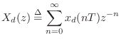
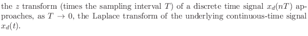
Relation to the z Transform
The Laplace transform is used to analyze continuous-time
systems. Its discrete-time counterpart is the  transform:
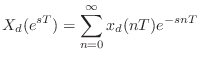
If we define

, the
transform becomes proportional to the
Laplace transform of a sampled continuous-time
signal:
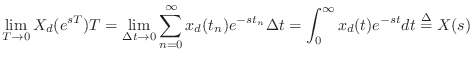
As the
sampling interval 
goes to zero, we have
where

and
.
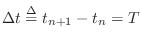
In summary,
Note that the plane and  plane are generally related by
In particular, the discrete-time frequency axis
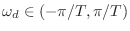
and
continuous-time frequency axis
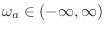
are related
by
For the mapping
from the
plane to the
plane to be invertible, it is necessary that

be zero for all

. If this is true, we say

is
bandlimited to half the sampling rate. As is well known, this
condition is necessary to prevent
aliasing when
sampling the
continuous-time signal
at the rate

to produce

,
(see [
84, Appendix G]).
Next Section: Laplace Transform TheoremsPrevious Section: Analytic Continuation