


Series Second-Order Sections
For many filter types, such as lowpass, highpass, and bandpass filters, a good choice of implementation structure is often series second-order sections. In fixed-point applications, the ordering of the sections can be important.
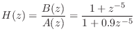
The matlab function tf2sos10.5 converts from ``transfer function form'',
![]() , to series ``second-order-section'' form.
For example, the line
, to series ``second-order-section'' form.
For example, the line
BAMatrix = tf2sos(B,A);converts the real filter specified by polynomial vectors B and A to a series of second-order sections (biquads) specified by the rows of BAMatrix. Each row of BAMatrix is of the form
function [sos,g] = tf2sos(B,A)
[z,p,g]=tf2zp(B(:)',A(:)'); % Direct form to (zeros,poles,gain)
sos=zp2sos(z,p,g); % (z,p,g) to series second-order sections
Matlab Example
The following matlab example expands the filter
B=[1 0 0 0 0 1];
A=[1 0 0 0 0 .9];
[sos,g] = tf2sos(B,A)
sos =
   1.00000   0.61803   1.00000   1.00000   0.60515   0.95873
   1.00000  -1.61803   1.00000   1.00000  -1.58430   0.95873
   1.00000   1.00000  -0.00000   1.00000   0.97915  -0.00000

g = 1
The g parameter is an input (or output) scale factor; for this filter, it was not needed. Thus, in this example we obtained the following filter factorization:
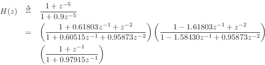
Note that the first two sections are second-order, while the third is first-order (when coefficients are rounded to five digits of precision after the decimal point).
In addition to tf2sos, tf2zp, and zp2sos discussed above, there are also functions sos2zp and sos2tf, which do the obvious conversion in both Matlab and Octave.10.6 The sos2tf function can be used to check that the second-order factorization is accurate:
% Numerically challenging "clustered roots" example:
[B,A] = zp2tf(ones(10,1),0.9*ones(10,1),1);
[sos,g] = tf2sos(B,A);
[Bh,Ah] = sos2tf(sos,g);
format long;
disp(sprintf('Relative L2 numerator error: %g',...
	norm(Bh-B)/norm(B)));
% Relative L2 numerator error: 1.26558e-15
disp(sprintf('Relative L2 denominator error: %g',...
	norm(Ah-A)/norm(A)));
% Relative L2 denominator error: 1.65594e-15
Thus, in this test, the original direct-form filter is compared with
one created from the second-order sections. Such checking should be
done for high-order filters, or filters having many poles and/or zeros
close together, because the polynomial factorization used to find the
poles and zeros can fail numerically. Moreover, the stability of the
factors should be checked individually.
Next Section:
Parallel First and/or Second-Order Sections
Previous Section:
Numerical Robustness of TDF-II


