


Parallel First and/or Second-Order Sections
Instead of breaking up a filter into a series of second-order
sections, as discussed in the previous section, we can break the
filter up into a parallel sum of first and/or second-order
sections. Parallel sections are based directly on the partial
fraction expansion (PFE) of the filter transfer function discussed in
§6.8. As discussed in §6.8.3, there is additionally an
FIR part when the order of the transfer-function denominator
does not exceed that of the numerator (i.e., when the transfer function
is not strictly proper). The most general case of a PFE, valid
for any finite-order transfer function, was given by Eq.![]() (6.19),
repeated here for convenience:
(6.19),
repeated here for convenience:
where
The FIR part ![]() is typically realized as a tapped delay line, as
shown in Fig.5.5.
is typically realized as a tapped delay line, as
shown in Fig.5.5.
First-Order Complex Resonators
For distinct poles, the recursive terms in the complete partial
fraction expansion of Eq.![]() (9.2) can be realized as a parallel sum
of complex one-pole filter
sections, thereby producing a parallel complex resonator filter
bank. Complex resonators are efficient for processing complex input
signals, and they are especially easy to work with. Note that a
complex resonator bank is similarly obtained by implementing a
diagonalized state-space model [Eq.
(9.2) can be realized as a parallel sum
of complex one-pole filter
sections, thereby producing a parallel complex resonator filter
bank. Complex resonators are efficient for processing complex input
signals, and they are especially easy to work with. Note that a
complex resonator bank is similarly obtained by implementing a
diagonalized state-space model [Eq.![]() (G.22)].
(G.22)].
Real Second-Order Sections
In practice, however, signals are typically real-valued functions of
time. As a result, for real filters (§5.1),
it is typically more efficient computationally to combine
complex-conjugate one-pole sections together to form real second-order
sections (two poles and one zero each, in general). This process was
discussed in §6.8.1, and the resulting transfer function of
each second-order section becomes
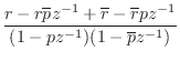
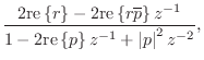
where
When the two poles of a real second-order section are complex, they
form a complex-conjugate pair, i.e., they are located at
![]() in the
in the ![]() plane, where
plane, where ![]() is the modulus of either
pole, and
is the modulus of either
pole, and ![]() is the angle of either pole. In this case, the
``resonance-tuning coefficient'' in Eq.
is the angle of either pole. In this case, the
``resonance-tuning coefficient'' in Eq.![]() (9.3) can be expressed as
(9.3) can be expressed as
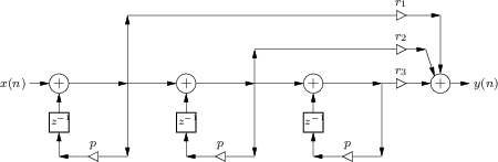
Figures 3.25 and 3.26 (p. ![]() ) illustrate filter realizations
consisting of one first-order and two second-order filter sections in
parallel.
) illustrate filter realizations
consisting of one first-order and two second-order filter sections in
parallel.
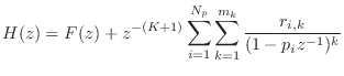
Implementation of Repeated Poles
Fig.9.5 illustrates an efficient implementation of terms due to a repeated pole with multiplicity three, contributing the additive terms
Next Section:
Formant Filtering Example
Previous Section:
Series Second-Order Sections


