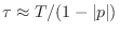
A useful approximate formula giving the decay
time-constant9.4  (in
seconds) in terms of a pole radius
(in
seconds) in terms of a pole radius  is
is
 |
(9.8) |
where

denotes the
sampling interval in seconds, and we assume

.
The exact relation between and  is obtained by sampling an
exponential decay:
is obtained by sampling an
exponential decay:
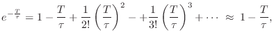
Thus, setting

yields
Expanding the right-hand side in a
Taylor series and neglecting terms
higher than first order gives
which derives

. Solving for
then gives
Eq.

(
8.8). From its derivation, we see that the approximation is
valid for
. Thus, as long as the
impulse response of a pole

``rings'' for many samples, the formula
should well estimate the time-constant of decay in seconds. The
time-constant estimate in
samples is of course

. For
higher-order systems, the approximate
decay time is
, where

is the largest pole
magnitude (closest to the unit circle) in the (stable) system.
Next Section: Unstable Poles--Unit Circle ViewpointPrevious Section: Bandwidth of One Pole