Aliasing of Sampled Signals

This section quantifies aliasing in the general case. This result is then used in the proof of the sampling theorem in the next section.

It is well known that when a continuous-time signal contains energy at a frequency higher than half the sampling rate , sampling at samples per second causes that energy to alias to a lower frequency. If we write the original frequency as $f = f_s/2 + \epsilon$ , then the new aliased frequency is $f_a = f_s/2 - \epsilon$ , for $\epsilon\leq f_s/2$ . This phenomenon is also called ``folding'', since is a ``mirror image'' of about . As we will see, however, this is not a complete description of aliasing, as it only applies to real signals. For general (complex) signals, it is better to regard the aliasing due to sampling as a summation over all spectral ``blocks'' of width .

Continuous-Time Aliasing Theorem

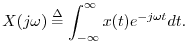
Let denote any continuous-time signal having a Fourier Transform (FT)

$\displaystyle X(j\omega)\isdef \int_{-\infty}^\infty x(t) e^{-j\omega t} dt.$

Let

$\displaystyle x_d(n) \isdef x(nT), \quad n=\ldots,-2,-1,0,1,2,\ldots,$

denote the samples of

at uniform intervals of

seconds, and denote its Discrete-Time Fourier Transform (DTFT) by

$\displaystyle X_d(e^{j\theta})\isdef \sum_{n=-\infty}^\infty x_d(n) e^{-j\theta n}.$

Then the spectrum

of the sampled signal

is related to the spectrum

of the original continuous-time signal

$\displaystyle X_d(e^{j\theta}) = \frac{1}{T} \sum_{m=-\infty}^\infty X\left[j\left(\frac{\theta}{T} + m\frac{2\pi}{T}\right)\right].$

The terms in the above sum for $m\neq 0$ are called aliasing terms. They are said to alias into the base band $[-\pi/T,\pi/T]$ . Note that the summation of a spectrum with aliasing components involves addition of complex numbers; therefore, aliasing components can be removed only if both their amplitude and phase are known.

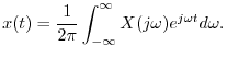
Proof: Writing as an inverse FT gives

$\displaystyle x(t) = \frac{1}{2\pi}\int_{-\infty}^\infty X(j\omega) e^{j\omega t} d\omega.$

Writing

as an inverse DTFT gives

$\displaystyle x_d(n) = \frac{1}{2\pi}\int_{-\pi}^\pi X_d(e^{j\theta}) e^{j \theta t} d\theta$

where $\theta \isdef 2\pi \omega_d T$ denotes the normalized discrete-time frequency variable.

The inverse FT can be broken up into a sum of finite integrals, each of length $\Omega_s \isdef 2\pi f_s= 2\pi/T$ , as follows:

$\begin{eqnarray*} x(t) &=& \frac{1}{2\pi}\int_{-\infty}^\infty X(j\omega) e^{j\o... ...y X\left(j\omega + j m\Omega_s \right) e^{j\Omega_s m t} d\omega \end{eqnarray*}$

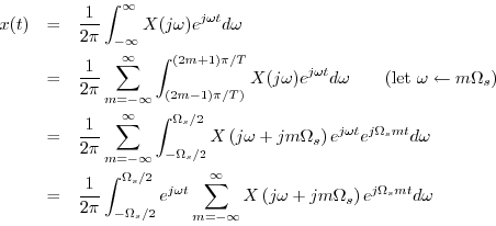
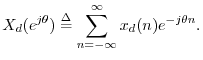
Let us now sample this representation for at to obtain $x_d(n) \isdef x(nT)$ , and we have

$\begin{eqnarray*} x_d(n) &=& \frac{1}{2\pi}\int_{-\Omega_s /2}^{\Omega_s /2} e^{... ..._{m=-\infty}^\infty X\left(j\omega + j m\Omega_s \right) d\omega \end{eqnarray*}$

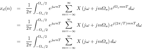
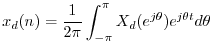
since and are integers. Normalizing frequency as $\theta^\prime = \omega T$ yields

$\displaystyle x_d(n) = \frac{1}{2\pi}\int_{-\pi}{\pi} e^{j\theta^\prime n} \f... ...t(\frac{\theta^\prime }{T} + m\frac{2\pi}{T}\right) \right] d\theta^\prime .$