


Introduction to Sampling
Inside computers and modern ``digital'' synthesizers, (as well as music CDs), sound is sampled into a stream of numbers. Each sample can be thought of as a number which specifies the positionD.2of a loudspeaker at a particular instant. When sound is sampled, we call it digital audio. The sampling rate used for CDs nowadays is 44,100 samples per second. That means when you play a CD, the speakers in your stereo system are moved to a new position 44,100 times per second, or once every 23 microseconds. Controlling a speaker this fast enables it to generate any sound in the human hearing range because we cannot hear frequencies higher than around 20,000 cycles per second, and a sampling rate more than twice the highest frequency in the sound guarantees that exact reconstruction is possible from the samples.
Reconstruction from Samples--Pictorial Version
Figure D.1 shows how a sound is reconstructed from its samples. Each sample can be considered as specifying the scaling and location of a sinc function. The discrete-time signal being interpolated in the figure is a digital rectangular pulse:
![\includegraphics[width=\twidth]{eps/SincSum}](http://www.dsprelated.com/josimages_new/mdft/img1765.png) |
Notice that each sinc function passes through zero at every sample instant but the one it is centered on, where it passes through 1.
The Sinc Function
![\includegraphics[width=\twidth]{eps/Sinc}](http://www.dsprelated.com/josimages_new/mdft/img1768.png)
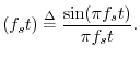
The sinc function, or cardinal sine function, is the famous ``sine x over x'' curve, and is illustrated in Fig.D.2. For bandlimited interpolation of discrete-time signals, the ideal interpolation kernel is proportional to the sinc function
Reconstruction from Samples--The Math
Let
![]() denote the
denote the ![]() th sample of the original
sound
th sample of the original
sound ![]() , where
, where ![]() is time in seconds. Thus,
is time in seconds. Thus, ![]() ranges over the
integers, and
ranges over the
integers, and ![]() is the sampling interval in seconds. The
sampling rate in Hertz (Hz) is just the reciprocal of the
sampling period,
i.e.,
is the sampling interval in seconds. The
sampling rate in Hertz (Hz) is just the reciprocal of the
sampling period,
i.e.,
To avoid losing any information as a result of sampling, we must
assume ![]() is bandlimited to less than half the sampling
rate. This means there can be no energy in
is bandlimited to less than half the sampling
rate. This means there can be no energy in ![]() at frequency
at frequency
![]() or above. We will prove this mathematically when we prove
the sampling theorem in §D.3 below.
or above. We will prove this mathematically when we prove
the sampling theorem in §D.3 below.
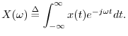
Let ![]() denote the Fourier transform of
denote the Fourier transform of ![]() , i.e.,
, i.e.,
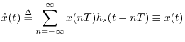
The reconstruction of a sound from its samples can thus be interpreted as follows: convert the sample stream into a weighted impulse train, and pass that signal through an ideal lowpass filter which cuts off at half the sampling rate. These are the fundamental steps of digital to analog conversion (DAC). In practice, neither the impulses nor the lowpass filter are ideal, but they are usually close enough to ideal that one cannot hear any difference. Practical lowpass-filter design is discussed in the context of bandlimited interpolation [72].
Next Section:
Aliasing of Sampled Signals
Previous Section:
The Uncertainty Principle


