


Sampling Theorem
Let ![]() denote any continuous-time signal having a continuous Fourier transform
denote any continuous-time signal having a continuous Fourier transform
Proof: From the continuous-time aliasing theorem (§D.2), we
have that the discrete-time spectrum
![]() can be written in
terms of the continuous-time spectrum
can be written in
terms of the continuous-time spectrum
![]() as
as
![$\displaystyle X_d(e^{j\omega_d T}) = \frac{1}{T} \sum_{m=-\infty}^\infty X[j(\omega_d +m\Omega_s )]
$](http://www.dsprelated.com/josimages_new/mdft/img1807.png)
To reconstruct ![]() from its samples
from its samples ![]() , we may simply take
the inverse Fourier transform of the zero-extended DTFT, because
, we may simply take
the inverse Fourier transform of the zero-extended DTFT, because
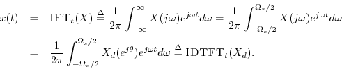
By expanding
![]() as the DTFT of the samples
as the DTFT of the samples ![]() , the
formula for reconstructing
, the
formula for reconstructing ![]() as a superposition of weighted sinc
functions is obtained (depicted in Fig.D.1):
as a superposition of weighted sinc
functions is obtained (depicted in Fig.D.1):

where we defined
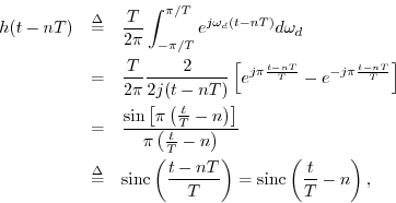
or
The ``sinc function'' is defined with where sinc
We have shown that when ![]() is bandlimited to less than half the
sampling rate, the IFT of the zero-extended DTFT of its samples
is bandlimited to less than half the
sampling rate, the IFT of the zero-extended DTFT of its samples
![]() gives back the original continuous-time signal
gives back the original continuous-time signal ![]() .
This completes the proof of the
sampling theorem.
.
This completes the proof of the
sampling theorem.
![]()
Conversely, if ![]() can be reconstructed from its samples
can be reconstructed from its samples
![]() , it must be true that
, it must be true that ![]() is bandlimited to
is bandlimited to
![]() , since a sampled signal only supports frequencies up
to
, since a sampled signal only supports frequencies up
to ![]() (see §D.4 below). While a real digital signal
(see §D.4 below). While a real digital signal
![]() may have energy at half the sampling rate (frequency
may have energy at half the sampling rate (frequency ![]() ),
the phase is constrained to be either 0 or
),
the phase is constrained to be either 0 or ![]() there, which is why
this frequency had to be excluded from the sampling theorem.
there, which is why
this frequency had to be excluded from the sampling theorem.
A one-line summary of the essence of the sampling-theorem proof is
The sampling theorem is easier to show when applied to sampling-rate
conversion in discrete-time, i.e., when simple downsampling of a
discrete time signal is being used to reduce the sampling rate by an
integer factor. In analogy with the continuous-time aliasing theorem
of §D.2, the downsampling theorem (§7.4.11)
states that downsampling a digital signal by an integer factor ![]() produces a digital signal whose spectrum can be calculated by
partitioning the original spectrum into
produces a digital signal whose spectrum can be calculated by
partitioning the original spectrum into ![]() equal blocks and then
summing (aliasing) those blocks. If only one of the blocks is
nonzero, then the original signal at the higher sampling rate is
exactly recoverable.
equal blocks and then
summing (aliasing) those blocks. If only one of the blocks is
nonzero, then the original signal at the higher sampling rate is
exactly recoverable.
Next Section:
Appendix: Frequencies Representable by a Geometric Sequence
Previous Section:
Aliasing of Sampled Signals


