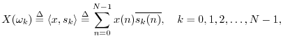
The Discrete Fourier Transform (DFT)
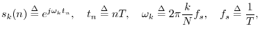
Given a signal
, its DFT is defined
by6.3
![$\displaystyle X(\omega_k) \isdef \left<x,s_k\right> \isdef \sum_{n=0}^{N-1}x(n) \overline{s_k(n)},
\quad k=0,1,2,\ldots,N-1,
$](http://www.dsprelated.com/josimages_new/mdft/img1037.png)
![$\displaystyle s_k(n)\isdef e^{j\omega_k t_n},
\quad t_n\isdef nT,
\quad \omega_k\isdef 2\pi\frac{k}{N}f_s,
\quad f_s\isdef \frac{1}{T},
$](http://www.dsprelated.com/josimages_new/mdft/img1038.png)
![$\displaystyle \zbox {X(\omega_k) \isdef \sum_{n=0}^{N-1}x(n) e^{-j\frac{2\pi k n}{N}},
\quad k=0,1,2,\ldots,N-1.}
$](http://www.dsprelated.com/josimages_new/mdft/img1039.png)
![$ X$](http://www.dsprelated.com/josimages_new/mdft/img55.png)
![$ x$](http://www.dsprelated.com/josimages_new/mdft/img25.png)
![$ X(\omega_k)$](http://www.dsprelated.com/josimages_new/mdft/img680.png)
![$ k$](http://www.dsprelated.com/josimages_new/mdft/img20.png)
![$ \omega_k$](http://www.dsprelated.com/josimages_new/mdft/img677.png)
![$ k$](http://www.dsprelated.com/josimages_new/mdft/img20.png)
![$ X(\omega_k)$](http://www.dsprelated.com/josimages_new/mdft/img680.png)
![$ x$](http://www.dsprelated.com/josimages_new/mdft/img25.png)
![$ k$](http://www.dsprelated.com/josimages_new/mdft/img20.png)
![$ s_k$](http://www.dsprelated.com/josimages_new/mdft/img96.png)
![$ N$](http://www.dsprelated.com/josimages_new/mdft/img35.png)
![$ x$](http://www.dsprelated.com/josimages_new/mdft/img25.png)
![$ s_k$](http://www.dsprelated.com/josimages_new/mdft/img96.png)
![$\displaystyle \frac{\left<x,s_k\right>}{\left\Vert\,s_k\,\right\Vert^2} = \frac{X(\omega_k)}{N}.
$](http://www.dsprelated.com/josimages_new/mdft/img1040.png)
![$ x$](http://www.dsprelated.com/josimages_new/mdft/img25.png)
![$ s_k$](http://www.dsprelated.com/josimages_new/mdft/img96.png)
![$\displaystyle {\bf P}_{s_k}(x) = \frac{X(\omega_k)}{N} s_k.
$](http://www.dsprelated.com/josimages_new/mdft/img1041.png)
![$ \{s_k\}$](http://www.dsprelated.com/josimages_new/mdft/img1042.png)
![$ {\bf C}^N$](http://www.dsprelated.com/josimages_new/mdft/img75.png)
![$\displaystyle x = \sum_{k=0}^{N-1}\frac{X(\omega_k)}{N} s_k,
$](http://www.dsprelated.com/josimages_new/mdft/img1043.png)
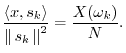
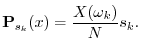
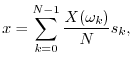
In summary, the DFT is proportional to the set of coefficients of projection onto the sinusoidal basis set, and the inverse DFT is the reconstruction of the original signal as a superposition of its sinusoidal projections. This basic ``architecture'' extends to all linear orthogonal transforms, including wavelets, Fourier transforms, Fourier series, the discrete-time Fourier transform (DTFT), and certain short-time Fourier transforms (STFT). See Appendix B for some of these.
We have defined the DFT from a geometric signal theory point of view, building on the preceding chapter. See §7.1.1 for notation and terminology associated with the DFT.
Next Section:
Frequencies in the ``Cracks''
Previous Section:
An Orthonormal Sinusoidal Set