Hann-Windowed Complex Sinusoid

In this example, we'll perform spectrum analysis on a complex sinusoid having only a single positive frequency. We'll use the Hann window (also known as the Hanning window) which does not have as much sidelobe suppression as the Blackman window, but its main lobe is narrower. Its sidelobes ``roll off'' very quickly versus frequency. Compare with the Blackman window results to see if you can see these differences.

The Matlab script for synthesizing and plotting the Hann-windowed sinusoid is given below:

% Analysis parameters:
M = 31;         % Window length
N = 64;         % FFT length (zero padding factor near 2)

% Signal parameters:
wxT = 2*pi/4;   % Sinusoid frequency (rad/sample)
A = 1;          % Sinusoid amplitude
phix = 0;       % Sinusoid phase

% Compute the signal x:
n = [0:N-1];    % time indices for sinusoid and FFT
x = A * exp(j*wxT*n+phix); % complex sine [1,j,-1,-j...]

% Compute Hann window:
nm = [0:M-1];   % time indices for window computation
% Hann window = "raised cosine", normalization (1/M)
% chosen to give spectral peak magnitude at 1/2:
w = (1/M) * (cos((pi/M)*(nm-(M-1)/2))).^2;

wzp = [w,zeros(1,N-M)]; % zero-pad out to the length of x
xw = x .* wzp;          % apply the window w to signal x

figure(1);
subplot(1,1,1);

% Display real part of windowed signal and Hann window
plot(n,wzp,'-k'); hold on; plot(n,real(xw),'*k'); hold off;
title(['Hann Window and Windowed, Zero-Padded, ',...
       'Sinusoid (Real Part)']);
xlabel('Time (samples)'); ylabel('Amplitude');

The resulting plot of the Hann window and its use on sinusoidal data are shown in Fig.8.7.

**Figure 8.7:** A length 31 Hann window (``raised cosine'') overlaid with the real part of the Hann-windowed complex sinusoid. Zero-padding is also shown. The sampled sinusoid is plotted using `*' with no connecting interpolation lines. You must now imagine the continuous real sinusoid (windowed) threading through the asterisks.
$\includegraphics[width=\twidth]{eps/hanning}$

Hann Window Spectrum Analysis Results

Finally, the Matlab for computing the DFT of the Hann-windowed complex sinusoid and plotting the results is listed below. To help see the full spectrum, we also compute a heavily interpolated spectrum (via zero padding as before) which we'll draw using solid lines.

% Compute the spectrum and its alternative forms:
Xw = fft(xw);              % FFT of windowed data
fn = [0:1.0/N:1-1.0/N];    % Normalized frequency axis
spec = 20*log10(abs(Xw));  % Spectral magnitude in dB
% Since the nulls can go to minus infinity, clip at -100 dB:
spec = max(spec,-100*ones(1,length(spec)));
phs = angle(Xw);           % Spectral phase in radians
phsu = unwrap(phs);        % Unwrapped spectral phase

% Compute heavily interpolated versions for comparison:
Nzp = 16;                   % Zero-padding factor
Nfft = N*Nzp;               % Increased FFT size
xwi = [xw,zeros(1,Nfft-N)]; % New zero-padded FFT buffer
Xwi = fft(xwi);             % Compute interpolated spectrum
fni = [0:1.0/Nfft:1.0-1.0/Nfft]; % Normalized freq axis
speci = 20*log10(abs(Xwi)); % Interpolated spec mag (dB)
speci = max(speci,-100*ones(1,length(speci))); % clip
phsi = angle(Xwi);          % Interpolated phase
phsiu = unwrap(phsi);       % Unwrapped interpolated phase

figure(1);
subplot(2,1,1);

plot(fn,abs(Xw),'*k'); hold on;
plot(fni,abs(Xwi),'-k'); hold off;
title('Spectral Magnitude');
xlabel('Normalized Frequency (cycles per sample))');
ylabel('Amplitude (linear)');

subplot(2,1,2);

% Same thing on a dB scale
plot(fn,spec,'*k'); hold on; plot(fni,speci,'-k'); hold off;
title('Spectral Magnitude (dB)');
xlabel('Normalized Frequency (cycles per sample))');
ylabel('Magnitude (dB)');

cmd = ['print -deps ', 'specmag.eps']; disp(cmd); eval(cmd);
disp 'pausing for RETURN (check the plot). . .'; pause

figure(1);
subplot(2,1,1);
plot(fn,phs,'*k'); hold on; plot(fni,phsi,'-k'); hold off;
title('Spectral Phase');
xlabel('Normalized Frequency (cycles per sample))');
ylabel('Phase (rad)'); grid;
subplot(2,1,2);
plot(fn,phsu,'*k'); hold on; plot(fni,phsiu,'-k'); hold off;
title('Unwrapped Spectral Phase');
xlabel('Normalized Frequency (cycles per sample))');
ylabel('Phase (rad)'); grid;
cmd = ['print -deps ', 'specphs.eps']; disp(cmd); eval(cmd);

Figure 8.8 shows the spectral magnitude and Fig.8.9 the spectral phase.

**Figure 8.8:** Spectral magnitude on linear (top) and dB (bottom) scales.
$\includegraphics[width=\twidth]{eps/specmag}$

There are no negative-frequency components in Fig.8.8 because we are analyzing a complex sinusoid $x=[1,j,-1,-j,1,j,\ldots\,]$ , which has frequency only, with no component at .

Notice how difficult it would be to correctly interpret the shape of the ``sidelobes'' without zero padding. The asterisks correspond to a zero-padding factor of 2, already twice as much as needed to preserve all spectral information faithfully, but not enough to clearly outline the sidelobes in a spectral magnitude plot.

Spectral Phase

As for the phase of the spectrum, what do we expect? We have chosen the sinusoid phase offset to be zero. The window is causal and symmetric about its middle. Therefore, we expect a linear phase term with slope samples (as discussed in connection with the shift theorem in §7.4.4). Also, the window transform has sidelobes which cause a phase of $\pi$ radians to switch in and out. Thus, we expect to see samples of a straight line (with slope samples) across the main lobe of the window transform, together with a switching offset by $\pi$ in every other sidelobe away from the main lobe, starting with the immediately adjacent sidelobes.

In Fig.8.9(a), we can see the negatively sloped line across the main lobe of the window transform, but the sidelobes are hard to follow. Even the unwrapped phase in Fig.8.9(b) is not as clear as it could be. This is because a phase jump of $\pi$ radians and $-\pi$ radians are equally valid, as is any odd multiple of $\pi$ radians. In the case of the unwrapped phase, all phase jumps are by $+\pi$ starting near frequency . Figure 8.9(c) shows what could be considered the ``canonical'' unwrapped phase for this example: We see a linear phase segment across the main lobe as before, and outside the main lobe, we have a continuation of that linear phase across all of the positive sidelobes, and only a $\pi$ -radian deviation from that linear phase across the negative sidelobes. In other words, we see a straight linear phase at the desired slope interrupted by temporary jumps of $\pi$ radians. To obtain unwrapped phase of this type, the unwrap function needs to alternate the sign of successive phase-jumps by $\pi$ radians; this could be implemented, for example, by detecting jumps-by- $\pi$ to within some numerical tolerance and using a bit of state to enforce alternation of $+\pi$ with $-\pi$ .

To convert the expected phase slope from ``radians per (rad/sec)'' to ``radians per cycle-per-sample,'' we need to multiply by ``radians per cycle,'' or $2\pi$ . Thus, in Fig.8.9(c), we expect a slope of radians per unit normalized frequency, or radians per cycles-per-sample, and this looks about right, judging from the plot.

**Figure 8.9:** Spectral phase and two different phase unwrappings.
$\includegraphics{eps/% specphs-wrapped}$ Raw spectral phase and its interpolation 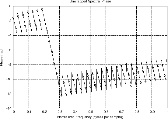$\includegraphics{eps/% specphs-unwrapped}$ Unwrapped spectral phase and its interpolation 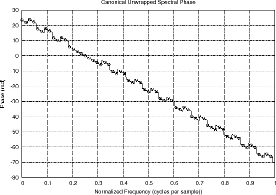$\includegraphics{eps/% specphs-unwrapped-linear}$ Canonically unwrapped spectral phase and its interpolation

Next Section:
Spectrogram of Speech
Previous Section:
Use of a Blackman Window