


The Length 2 DFT
The length ![]() DFT is particularly simple, since the basis sinusoids
are real:
DFT is particularly simple, since the basis sinusoids
are real:
The DFT sinusoid ![]() is a sampled constant signal, while
is a sampled constant signal, while ![]() is a
sampled sinusoid at half the sampling rate.
is a
sampled sinusoid at half the sampling rate.
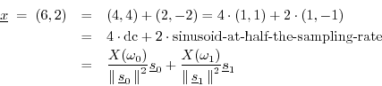
Figure 6.4 illustrates the graphical relationships for the length
![]() DFT of the signal
DFT of the signal
![]() .
.
![\includegraphics[width=\twidth]{eps/dft2}](http://www.dsprelated.com/josimages_new/mdft/img1077.png)
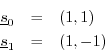
Analytically, we compute the DFT to be
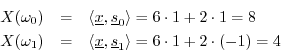
and the corresponding projections onto the DFT sinusoids are
Note the lines of orthogonal projection illustrated in the figure. The
``time domain'' basis consists of the vectors
![]() , and the
orthogonal projections onto them are simply the coordinate axis projections
, and the
orthogonal projections onto them are simply the coordinate axis projections
![]() and
and ![]() . The ``frequency domain'' basis vectors are
. The ``frequency domain'' basis vectors are
![]() , and they provide an orthogonal basis set that is rotated
, and they provide an orthogonal basis set that is rotated
![]() degrees relative to the time-domain basis vectors. Projecting
orthogonally onto them gives
degrees relative to the time-domain basis vectors. Projecting
orthogonally onto them gives
![]() and
and
![]() , respectively.
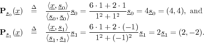
The original signal
, respectively.
The original signal
![]() can be
expressed either as the vector sum of its coordinate projections
(0,...,x(i),...,0), (a time-domain representation), or as the
vector sum of its projections onto the DFT sinusoids (a
frequency-domain representation of the time-domain signal
can be
expressed either as the vector sum of its coordinate projections
(0,...,x(i),...,0), (a time-domain representation), or as the
vector sum of its projections onto the DFT sinusoids (a
frequency-domain representation of the time-domain signal
![]() ).
Computing the coefficients of projection is essentially ``taking the
DFT,'' and constructing
).
Computing the coefficients of projection is essentially ``taking the
DFT,'' and constructing
![]() as the vector sum of its projections onto
the DFT sinusoids amounts to ``taking the inverse DFT.''
as the vector sum of its projections onto
the DFT sinusoids amounts to ``taking the inverse DFT.''
In summary, the oblique coordinates in Fig.6.4 are interpreted as follows:
Next Section:
Matrix Formulation of the DFT
Previous Section:
Normalized DFT


