


Sinusoidal Amplitude Modulation (AM)
It is instructive to study the modulation of one sinusoid by another. In this section, we will look at sinusoidal Amplitude Modulation (AM). The general AM formula is given by
In the case of sinusoidal AM, we have
Periodic amplitude modulation of this nature is often called the tremolo effect when
Let's analyze the second term of Eq.![]() (4.1) for the case of sinusoidal
AM with
(4.1) for the case of sinusoidal
AM with ![]() and
and
![]() :
:
An example waveform is shown in Fig.4.11 for
![\includegraphics[width=3.5in]{eps/sineamtd}](http://www.dsprelated.com/josimages_new/mdft/img494.png)
When ![]() is small (say less than
is small (say less than ![]() radians per second, or
10 Hz), the signal
radians per second, or
10 Hz), the signal ![]() is heard as a ``beating sine wave'' with
is heard as a ``beating sine wave'' with
![]() beats per second. The beat rate is
twice the modulation frequency because both the positive and negative
peaks of the modulating sinusoid cause an ``amplitude swell'' in
beats per second. The beat rate is
twice the modulation frequency because both the positive and negative
peaks of the modulating sinusoid cause an ``amplitude swell'' in
![]() . (One period of modulation--
. (One period of modulation--![]() seconds--is shown in
Fig.4.11.) The sign inversion during the negative peaks is not
normally audible.
seconds--is shown in
Fig.4.11.) The sign inversion during the negative peaks is not
normally audible.
Recall the trigonometric identity for a sum of angles:
![$\displaystyle x_m(t) \isdef \sin(\omega_m t)\sin(\omega_c t) = \frac{\cos[(\omega_m-\omega_c)t] - \cos[(\omega_m+\omega_c)t]}{2} \protect$](http://www.dsprelated.com/josimages_new/mdft/img505.png)
These two sinusoidal components at the sum and difference frequencies of the modulator and carrier are called side bands of the carrier wave at frequency
Equation (4.3) expresses ![]() as a ``beating sinusoid'', while
Eq.
as a ``beating sinusoid'', while
Eq.![]() (4.4) expresses as it two unmodulated sinusoids at
frequencies
(4.4) expresses as it two unmodulated sinusoids at
frequencies
![]() . Which case do we hear?
. Which case do we hear?
It turns out we hear ![]() as two separate tones (Eq.
as two separate tones (Eq.![]() (4.4))
whenever the side bands are resolved by the ear. As
mentioned in §4.1.2,
the ear performs a ``short time Fourier analysis'' of incoming sound
(the basilar membrane in the cochlea acts as a mechanical
filter bank). The
resolution of this filterbank--its ability to discern two
separate spectral peaks for two sinusoids closely spaced in
frequency--is determined by the
critical bandwidth of hearing
[45,76,87]. A critical
bandwidth is roughly 15-20% of the band's center-frequency, over most
of the audio range [71]. Thus, the side bands in
sinusoidal AM are heard as separate tones when they are both in the
audio range and separated by at least one critical bandwidth. When
they are well inside the same critical band, ``beating'' is heard. In
between these extremes, near separation by a critical-band, the
sensation is often described as ``roughness'' [29].
(4.4))
whenever the side bands are resolved by the ear. As
mentioned in §4.1.2,
the ear performs a ``short time Fourier analysis'' of incoming sound
(the basilar membrane in the cochlea acts as a mechanical
filter bank). The
resolution of this filterbank--its ability to discern two
separate spectral peaks for two sinusoids closely spaced in
frequency--is determined by the
critical bandwidth of hearing
[45,76,87]. A critical
bandwidth is roughly 15-20% of the band's center-frequency, over most
of the audio range [71]. Thus, the side bands in
sinusoidal AM are heard as separate tones when they are both in the
audio range and separated by at least one critical bandwidth. When
they are well inside the same critical band, ``beating'' is heard. In
between these extremes, near separation by a critical-band, the
sensation is often described as ``roughness'' [29].
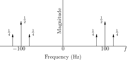
Example AM Spectra
Equation (4.4) can be used to write down the spectral representation of
![]() by inspection, as shown in Fig.4.12. In the example
of Fig.4.12, we have
by inspection, as shown in Fig.4.12. In the example
of Fig.4.12, we have ![]() Hz and
Hz and ![]() Hz,
where, as always,
Hz,
where, as always,
![]() . For comparison, the spectral
magnitude of an unmodulated
. For comparison, the spectral
magnitude of an unmodulated ![]() Hz sinusoid is shown in
Fig.4.6. Note in Fig.4.12 how each of the two
sinusoidal components at
Hz sinusoid is shown in
Fig.4.6. Note in Fig.4.12 how each of the two
sinusoidal components at ![]() Hz have been ``split'' into two
``side bands'', one
Hz have been ``split'' into two
``side bands'', one ![]() Hz higher and the other
Hz higher and the other ![]() Hz lower, that
is,
Hz lower, that
is,
![]() . Note also how the
amplitude of the split component is divided equally among its
two side bands.
. Note also how the
amplitude of the split component is divided equally among its
two side bands.

Recall that ![]() was defined as the second term of
Eq.
was defined as the second term of
Eq.![]() (4.1). The first term is simply the original unmodulated
signal. Therefore, we have effectively been considering AM with a
``very large'' modulation index. In the more general case of
Eq.
(4.1). The first term is simply the original unmodulated
signal. Therefore, we have effectively been considering AM with a
``very large'' modulation index. In the more general case of
Eq.![]() (4.1) with
(4.1) with ![]() given by Eq.
given by Eq.![]() (4.2), the magnitude of
the spectral representation appears as shown in Fig.4.13.
(4.2), the magnitude of
the spectral representation appears as shown in Fig.4.13.
Next Section:
Sinusoidal Frequency Modulation (FM)
Previous Section:
Plotting Complex Sinusoids versus Frequency


