


Checking the WDF against the Analog Equivalent Circuit
Let's check our result by comparing the transfer function from the input force to the force on the mass in both the discrete- and continuous-time cases.
For the discrete-time case, we have

We now need
![]() .
To simplify notation, define the two coefficients as
.
To simplify notation, define the two coefficients as

From Figure F.30, we can write
![\begin{eqnarray*}
F^{-}_3(z) &=& -a\left[F(z)-z^{-1}F^{-}_3(z)\right] + b\left[-...
...\,\,\quad
F^{-}_3(z) &=& -a\frac{F(z)}{1-(a-b)z^{-1}F^{-}_3(z)}
\end{eqnarray*}](http://www.dsprelated.com/josimages_new/pasp/img4987.png)
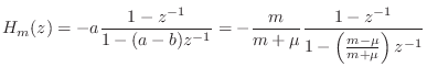
Thus, the desired transfer function is
We now wish to compare this result to the bilinear transform of the corresponding analog transfer function. From Figure F.27, we can recognize the mass and dashpot as voltage divider:
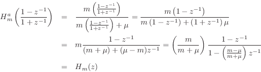
Thus, we have verified that the force transfer-function from the driving force to the mass is identical in the discrete- and continuous-time models, except for the bilinear transform frequency warping in the discrete-time case.
Next Section:
Oscillation Frequency
Previous Section:
A More Formal Derivation of the Wave Digital Force-Driven Mass


