


FDN and State Space Descriptions
When
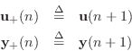
![]() in Eq.
in Eq.![]() (2.10), the FDN (Fig.2.28)
reduces to a normal state-space model (§1.3.7),
(2.10), the FDN (Fig.2.28)
reduces to a normal state-space model (§1.3.7),
The matrix
to follow normal convention for state-space form.
Thus, an FDN can be viewed as a generalized state-space model for a
class of ![]() th-order linear systems--``generalized'' in the sense
that unit delays are replaced by arbitrary delays. This
correspondence is valuable for analysis because tools for state-space
analysis are well known and included in many software libraries such
as with matlab.
th-order linear systems--``generalized'' in the sense
that unit delays are replaced by arbitrary delays. This
correspondence is valuable for analysis because tools for state-space
analysis are well known and included in many software libraries such
as with matlab.
Next Section:
Single-Input, Single-Output (SISO) FDN
Previous Section:
Time Varying Comb Filters


