


Feedback Delay Networks (FDN)
![\includegraphics[width=\twidth]{eps/FDNMIMO}](http://www.dsprelated.com/josimages_new/pasp/img529.png)
The FDN can be seen as a vector feedback comb filter,3.10obtained by replacing the delay line with a diagonal delay matrix
(defined in Eq.![]() (2.10) below), and replacing the feedback gain
(2.10) below), and replacing the feedback gain
![]() by the product of a diagonal matrix
by the product of a diagonal matrix
![]() times an orthogonal
matrix
times an orthogonal
matrix
![]() , as shown in
Fig.2.28 for
, as shown in
Fig.2.28 for ![]() . The time-update for this FDN can be written
as
. The time-update for this FDN can be written
as
![$\displaystyle \left[\begin{array}{c} x_1(n) \\ [2pt] x_2(n) \\ [2pt] x_3(n)\end...
...gin{array}{c} u_1(n) \\ [2pt] u_2(n) \\ [2pt] u_3(n)\end{array}\right] \protect$](http://www.dsprelated.com/josimages_new/pasp/img533.png)
with the outputs given by
![$\displaystyle \left[\begin{array}{c} y_1(n) \\ [2pt] y_2(n) \\ [2pt] y_3(n)\end...
...array}{c} x_1(n-M_1) \\ [2pt] x_2(n-M_2) \\ [2pt] x_3(n-M_3)\end{array}\right],$](http://www.dsprelated.com/josimages_new/pasp/img534.png) |
(3.7) |
or, in frequency-domain vector notation,
| (3.8) | |||
| (3.9) |
where
FDN and State Space Descriptions
When
![]() in Eq.
in Eq.![]() (2.10), the FDN (Fig.2.28)
reduces to a normal state-space model (§1.3.7),
(2.10), the FDN (Fig.2.28)
reduces to a normal state-space model (§1.3.7),
The matrix
to follow normal convention for state-space form.
Thus, an FDN can be viewed as a generalized state-space model for a
class of ![]() th-order linear systems--``generalized'' in the sense
that unit delays are replaced by arbitrary delays. This
correspondence is valuable for analysis because tools for state-space
analysis are well known and included in many software libraries such
as with matlab.
th-order linear systems--``generalized'' in the sense
that unit delays are replaced by arbitrary delays. This
correspondence is valuable for analysis because tools for state-space
analysis are well known and included in many software libraries such
as with matlab.
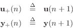
Single-Input, Single-Output (SISO) FDN
When there is only one input signal ![]() , the input vector
, the input vector
![]() in Fig.2.28 can be defined as the scalar input
in Fig.2.28 can be defined as the scalar input ![]() times a
vector of gains:
times a
vector of gains:
![\includegraphics[width=\twidth]{eps/FDNSISO}](http://www.dsprelated.com/josimages_new/pasp/img555.png)
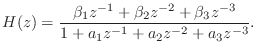
Note that when
![]() , this system is capable of realizing
any transfer function of the form
, this system is capable of realizing
any transfer function of the form
The more general case shown in Fig.2.29 can be handled in one of
two ways: (1) the matrices
![]() can be augmented
to order
can be augmented
to order
![]() such that the three delay lines are replaced
by
such that the three delay lines are replaced
by ![]() unit-sample delays, or (2) ordinary state-space analysis
may be generalized to non-unit delays, yielding
unit-sample delays, or (2) ordinary state-space analysis
may be generalized to non-unit delays, yielding
![$\displaystyle \mathbf{D}(z) \isdef \left[\begin{array}{ccc} z^{-M_1} & 0 & 0\\ [2pt] 0 & z^{-M_2} & 0\\ [2pt] 0 & 0 & z^{-M_3} \end{array}\right]. \protect$](http://www.dsprelated.com/josimages_new/pasp/img539.png)
In FDN reverberation applications,
![]() , where
, where
![]() is an orthogonal matrix, for reasons addressed below, and
is an orthogonal matrix, for reasons addressed below, and
![]() is a
diagonal matrix of lowpass filters, each having gain bounded by 1. In
certain applications, the subset of orthogonal matrices known as
circulant matrices have advantages [385].
is a
diagonal matrix of lowpass filters, each having gain bounded by 1. In
certain applications, the subset of orthogonal matrices known as
circulant matrices have advantages [385].
FDN Stability
Stability of the FDN is assured when some norm [451] of
the state vector
![]() decreases over time when the input signal is
zero [220, ``Lyapunov stability theory'']. That is, a
sufficient condition for FDN stability is
decreases over time when the input signal is
zero [220, ``Lyapunov stability theory'']. That is, a
sufficient condition for FDN stability is
for all
![$\displaystyle \mathbf{x}(n+1) = \mathbf{A}\left[\begin{array}{c} x_1(n-M_1) \\ [2pt] x_2(n-M_2) \\ [2pt] x_3(n-M_3)\end{array}\right].
$](http://www.dsprelated.com/josimages_new/pasp/img567.png)
for all
The matrix norm corresponding to any vector norm
![]() may be defined for the matrix
may be defined for the matrix
![]() as
as
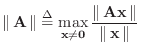
where
It can be shown [167] that the spectral norm of a matrix
![]() is given by the largest singular value of
is given by the largest singular value of
![]() (``
(``
![]() ''), and that this is equal to the
square-root of the largest eigenvalue of
''), and that this is equal to the
square-root of the largest eigenvalue of
![]() , where
, where
![]() denotes the matrix transpose of the real matrix
denotes the matrix transpose of the real matrix
![]() .3.11
.3.11
Since every orthogonal matrix
![]() has spectral norm
1,3.12 a wide variety of stable
feedback matrices can be parametrized as
has spectral norm
1,3.12 a wide variety of stable
feedback matrices can be parametrized as
![$\displaystyle {\bm \Gamma}= \left[ \begin{array}{cccc}
g_1 & 0 & \dots & 0\\
0...
...\\
0 & 0 & \dots & g_N
\end{array}\right], \quad \left\vert g_i\right\vert<1.
$](http://www.dsprelated.com/josimages_new/pasp/img587.png)
An alternative stability proof may be based on showing that an FDN is
a special case of a passive digital waveguide network (derived in
§C.15). This analysis reveals that the FDN is lossless if
and only if the feedback matrix
![]() has unit-modulus eigenvalues
and linearly independent eigenvectors.
has unit-modulus eigenvalues
and linearly independent eigenvectors.
Next Section:
Allpass Filters
Previous Section:
Comb Filters


