Finite-Difference Schemes (FDSs) aim to solve differential
equations by means of finite differences. For example, as discussed
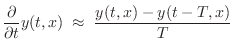
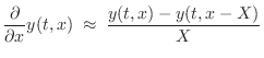
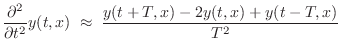
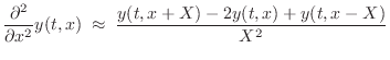
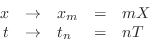
in §C.2, if  denotes the displacement in meters of a vibrating
string at time
denotes the displacement in meters of a vibrating
string at time  seconds and position
  meters, we may approximate
the first- and second-order partial derivatives by
meters, we may approximate
the first- and second-order partial derivatives by
where

denotes the time
sampling interval and

denotes the
spatial
sampling interval. Other types of finite-difference schemes
were derived in Chapter
7 (§
7.3.1), including a look at
frequency-domain properties. These
finite-difference approximations
to the partial derivatives may be used to compute solutions of
differential equations on a discrete grid:
Let us define an abbreviated notation for the grid variables
and consider the ideal
string wave equation (cf, §
C.1):
 |
(D.2) |
where

is a positive real constant (which turns out to be wave
propagation speed). Then, as derived in §
C.2, setting

and substituting the finite-difference approximations into
the ideal
wave equation leads to the relation
everywhere on the time-space grid (
i.e., for all

and

). Solving
for

in terms of displacement samples at earlier times yields an
explicit finite-difference scheme
for string displacement:
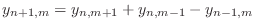 |
(D.3) |
The FDS is called
explicit because it was possible to solve for
the state at time
as a function of the state at earlier times (and
any other positions
). This allows it to be implemented as a time
recursion (or ``
digital filter'') which computes a solution at time
from solution samples at earlier times (and any spatial
positions). When an explicit FDS is not possible (
e.g., a non-
causal
filter is derived), the discretized differential equation is said to
define an
implicit FDS. An implicit FDS
can often be converted to an explicit FDS by a rotation of coordinates
[
55,
481].
Next Section: ConvergencePrevious Section: Non-Cylindrical Acoustic Tubes