


Terminated String Impedance
Note that the impedance of the terminated string, seen from one
of its endpoints, is not the same thing as the wave impedance
![]() of the string itself. If the string is infinitely
long, they are the same. However, when there are reflections,
they must be included in the impedance calculation, giving it an
imaginary part. We may say that the impedance has a ``reactive''
component. The driving-point impedance of a rigidly terminated string
is ``purely reactive,'' and may be called a reactance (§7.1).
If
of the string itself. If the string is infinitely
long, they are the same. However, when there are reflections,
they must be included in the impedance calculation, giving it an
imaginary part. We may say that the impedance has a ``reactive''
component. The driving-point impedance of a rigidly terminated string
is ``purely reactive,'' and may be called a reactance (§7.1).
If ![]() denotes the force at the driving-point of the
string and
denotes the force at the driving-point of the
string and ![]() denotes its velocity, then the driving-point
impedance is given by (§7.1)
denotes its velocity, then the driving-point
impedance is given by (§7.1)
Computational Savings
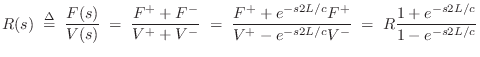
To illustrate how significant the computational savings can be,
consider the simulation of a ``damped guitar string'' model in
Fig.6.11. For simplicity, the length ![]() string is
rigidly terminated on both ends. Let the string be ``plucked'' by
initial conditions so that we need not couple an input mechanism to
the string. Also, let the output be simply the signal passing through
a particular delay element rather than the more realistic summation of
opposite elements in the bidirectional delay line. (A comb filter
corresponding to pluck position can be added in series later.)
string is
rigidly terminated on both ends. Let the string be ``plucked'' by
initial conditions so that we need not couple an input mechanism to
the string. Also, let the output be simply the signal passing through
a particular delay element rather than the more realistic summation of
opposite elements in the bidirectional delay line. (A comb filter
corresponding to pluck position can be added in series later.)
![\includegraphics[width=\twidth]{eps/fstring}](http://www.dsprelated.com/josimages_new/pasp/img1418.png) |
In this string simulator, there is a loop of delay containing
![]() samples where
samples where ![]() is the desired pitch of the string. Because
there is no input/output coupling, we may lump all of the losses at
a single point in the delay loop. Furthermore, the two reflecting
terminations (gain factors of
is the desired pitch of the string. Because
there is no input/output coupling, we may lump all of the losses at
a single point in the delay loop. Furthermore, the two reflecting
terminations (gain factors of ![]() ) may be commuted so as to cancel them.
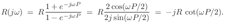
Finally, the right-going delay may be combined with the left-going delay to
give a single, length
) may be commuted so as to cancel them.
Finally, the right-going delay may be combined with the left-going delay to
give a single, length ![]() , delay line. The result of these inaudible
simplifications is shown in Fig. 6.12.
, delay line. The result of these inaudible
simplifications is shown in Fig. 6.12.
![\includegraphics[width=\twidth]{eps/fsstring}](http://www.dsprelated.com/josimages_new/pasp/img1421.png) |
If the sampling rate is ![]() kHz and the desired pitch is
kHz and the desired pitch is ![]() Hz, the loop delay equals
Hz, the loop delay equals ![]() samples. Since delay lines are
efficiently implemented as circular buffers, the cost of implementation is
normally dominated by the loss factors, each one requiring a multiply
every sample, in general. (Losses of the form
samples. Since delay lines are
efficiently implemented as circular buffers, the cost of implementation is
normally dominated by the loss factors, each one requiring a multiply
every sample, in general. (Losses of the form ![]() ,
,
![]() , etc., can be efficiently implemented using shifts and
adds.) Thus, the consolidation of loss factors has reduced computational
complexity by three orders of magnitude, i.e., by a factor of
, etc., can be efficiently implemented using shifts and
adds.) Thus, the consolidation of loss factors has reduced computational
complexity by three orders of magnitude, i.e., by a factor of
![]() in this case. However, the physical accuracy of the simulation has
not been compromised. In fact, the accuracy is improved because
the
in this case. However, the physical accuracy of the simulation has
not been compromised. In fact, the accuracy is improved because
the ![]() round-off errors per period arising from repeated multiplication
by
round-off errors per period arising from repeated multiplication
by ![]() have been replaced by a single round-off error per period
in the multiplication by
have been replaced by a single round-off error per period
in the multiplication by ![]() .
.
Next Section:
Stiff String Synthesis Models
Previous Section:
Animation of Moving String Termination and Digital Waveguide Models


