


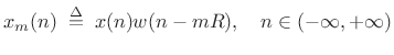
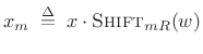
Overlap-Add Decomposition
Consider breaking an input signal ![]() into frames using a finite,
zero-phase, length
into frames using a finite,
zero-phase, length ![]() window
window ![]() . Then we may express the
. Then we may express the ![]() th
windowed data frame as
th
windowed data frame as
 |
(9.17) |
or
 |
(9.18) |
where

The hop size is the number of samples between the begin-times of adjacent frames. Specifically, it is the number of samples by which we advance each successive window.
Figure 8.8 shows an input signal (top) and three successive
windowed data frames using a length ![]() causal Hamming window and
50% overlap (
causal Hamming window and
50% overlap (![]() ).
).
![\includegraphics[width=\textwidth ]{eps/windsig}](http://www.dsprelated.com/josimages_new/sasp2/img1388.png)
For frame-by-frame spectral processing to work, we must be able to
reconstruct ![]() from the individual overlapping frames, ideally by
simply summing them in their original time positions. This can be
written as
from the individual overlapping frames, ideally by
simply summing them in their original time positions. This can be
written as
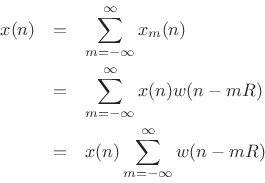
Hence,
![]() if and only if
if and only if
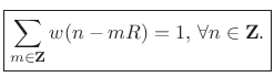 |
(9.19) |
This is the constant-overlap-add (COLA)9.6 constraint for the FFT analysis window
![\includegraphics[width=3.5in]{eps/cola}](http://www.dsprelated.com/josimages_new/sasp2/img1392.png)
Figure 8.9 illustrates the appearance of 50% overlap-add for
the Bartlett (triangular) window. The Bartlett window is clearly COLA
for a wide variety of hop sizes, such as ![]() ,
, ![]() , and so on,
provided
, and so on,
provided ![]() is an integer (otherwise the underlying continuous
triangular window must be resampled). However, when using windows
defined in a library, the COLA condition should be carefully checked.
For example, the following Matlab/Octave script shows that there
is a problem with the standard Hamming window:
is an integer (otherwise the underlying continuous
triangular window must be resampled). However, when using windows
defined in a library, the COLA condition should be carefully checked.
For example, the following Matlab/Octave script shows that there
is a problem with the standard Hamming window:
M = 33;          % window length
R = (M-1)/2;     % hop size
N = 3*M;         % overlap-add span
w = hamming(M);  % window
z = zeros(N,1);  plot(z,'-k');  hold on;  s = z;
for so=0:R:N-M
  ndx = so+1:so+M;        % current window location
  s(ndx) = s(ndx) + w;    % window overlap-add
  wzp = z; wzp(ndx) = w;  % for plot only
  plot(wzp,'--ok');       % plot just this window
end
plot(s,'ok');  hold off;  % plot window overlap-add
The figure produced by this matlab code is shown in Fig.8.10. As can be seen, the equal end-points sum to form an impulse in each frame of the overlap-add.
![\includegraphics[width=3.5in]{eps/tolaq}](http://www.dsprelated.com/josimages_new/sasp2/img1395.png)
The Matlab window functions (such as hamming) have an optional second argument which can be either 'symmetric' (the default), or 'periodic'. The periodic case is equivalent to
w = hamming(M+1); % symmetric case
w = w(1:M);       % delete last sample for periodic case
The periodic variant solves the non-constant overlap-add problem for even
w = hamming(M); % symmetric case
w(1) = w(1)/2;  % repair constant-overlap-add for R=(M-1)/2
w(M) = w(M)/2;
Since different window types may add or subtract 1 to/from
- hamming(M)

.54 - .46*cos(2*pi*(0:M-1)'/(M-1));
gives constant overlap-add for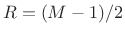 ,
,  , etc.,
when endpoints are divided by 2 or one endpoint is zeroed
, etc.,
when endpoints are divided by 2 or one endpoint is zeroed
- hanning(M)
.5*(1 - cos(2*pi*(1:M)'/(M+1)));
does not give constant overlap-add for
,
but does for 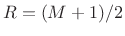
- blackman(M)
.42 - .5*cos(2*pi*m)' + .08*cos(4*pi*m)';
where m = (0:M-1)/(M-1), gives constant overlap-add for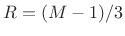 when
when  is odd and
  is an integer, and
  when
is even and
is integer.
when
is even and
is integer.
In summary, all windows obeying the constant-overlap-add constraint
will yield perfect reconstruction of the original signal ![]() from the
data frames
from the
data frames
![]() by overlap-add (OLA). There
is no constraint on window type, only that the window overlap-adds to
a constant for the hop size used. In particular,
by overlap-add (OLA). There
is no constraint on window type, only that the window overlap-adds to
a constant for the hop size used. In particular, ![]() always yields
a constant overlap-add for any window function. We will learn later
(§8.3.1) that there is also a simple frequency-domain test on
the window transform for the constant overlap-add property.
always yields
a constant overlap-add for any window function. We will learn later
(§8.3.1) that there is also a simple frequency-domain test on
the window transform for the constant overlap-add property.
To emphasize an earlier point, if simple time-invariant FIR filtering
is being implemented, and we don't need to work with the intermediate
STFT, it is most efficient to use the rectangular window with
hop size ![]() , and to set
, and to set ![]() , where
, where ![]() is the length of the
filter
is the length of the
filter ![]() and
and ![]() is a convenient FFT size. The optimum
is a convenient FFT size. The optimum ![]() for a
given
for a
given ![]() is an interesting exercise to work out.
is an interesting exercise to work out.
Next Section:
COLA Examples
Previous Section:
FFT versus Direct Convolution


