


Impulse Trains
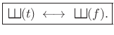
The impulse signal ![]() (defined in §B.10)
has a constant Fourier transform:
(defined in §B.10)
has a constant Fourier transform:
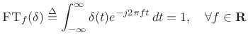 |
(B.43) |
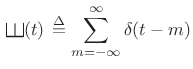
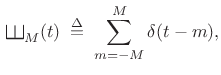
An impulse train can be defined as a sum of shifted impulses:
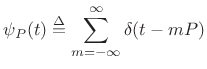 |
(B.44) |
Here,
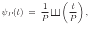
where
 |
(B.46) |
Note that the scaling by
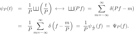
We will now show that
 |
(B.47) |
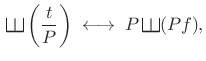
That is, the Fourier transform of the normalized impulse train
 |
(B.48) |
so that the
Thus, the ![]() -periodic impulse train transforms to a
-periodic impulse train transforms to a ![]() -periodic
impulse train, in which each impulse contains area
-periodic
impulse train, in which each impulse contains area ![]() :
:
 |
(B.49) |
Proof:
Let's set up a limiting construction by defining
 |
(B.50) |
so that
![\begin{eqnarray*}
\hbox{\sc FT}_f(\,\raisebox{0.8em}{\rotatebox{-90}{\resizebox{1em}{1em}{\ensuremath{\exists}}}}_M) &\isdef & \hbox{\sc FT}_f\left[\sum_{m=-M}^M \hbox{\sc Shift}_{m}(\delta)\right]\\
&=& \sum_{m=-M}^M \hbox{\sc FT}_f[\hbox{\sc Shift}_{m}(\delta)] \eqsp \sum_{m=-M}^M e^{-j2\pi f m}.
\end{eqnarray*}](http://www.dsprelated.com/josimages_new/sasp2/img2506.png)
Using the closed form of a geometric series,
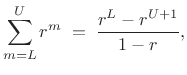 |
(B.51) |
with
![\begin{eqnarray*}
\hbox{\sc FT}_f(\,\raisebox{0.8em}{\rotatebox{-90}{\resizebox{1em}{1em}{\ensuremath{\exists}}}}_M)
&=& \frac{e^{j2\pi f M } - e^{-j2\pi f M } e^{-j2\pi f }}{1-e^{-j2\pi f }}\\ [10pt]
&=& \frac{e^{-j\pi f}}{e^{-j\pi f}}
\cdot
\frac{e^{j\pi f (2M+1) } - e^{-j\pi f (2M+1) }}{e^{j\pi f}-e^{-j\pi f}}\\ [10pt]
&=& \frac{\sin[\pi f (2M+1) ]}{\sin(\pi f)}\\ [5pt]
&\isdef & (2M+1)\,\hbox{asinc}_{2M+1}(2\pi f )
\end{eqnarray*}](http://www.dsprelated.com/josimages_new/sasp2/img2509.png)
where we have used the definition of
![]() given in
Eq.
given in
Eq.![]() (3.5) of §3.1. As we would
expect from basic sampling theory, the Fourier transform of the
sampled rectangular pulse is an aliased sinc function.
Figure 3.2 illustrates one period
(3.5) of §3.1. As we would
expect from basic sampling theory, the Fourier transform of the
sampled rectangular pulse is an aliased sinc function.
Figure 3.2 illustrates one period
![]() for
for
![]() .
.
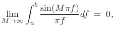
The proof can be completed by expressing the aliased sinc function as
a sum of regular sinc functions, and using linearity of the Fourier
transform to distribute
![]() over the sum, converting each sinc
function into an impulse, in the limit, by §B.13:
over the sum, converting each sinc
function into an impulse, in the limit, by §B.13:
![\begin{eqnarray*}
(2M+1)\,\hbox{asinc}_{2M+1}(2\pi f) &\isdef &
\frac{\sin[\pi f (2M+1) ]}{\sin(\pi f)}\\ [5pt]
&=& \sum_{k=-\infty}^{\infty} \mbox{sinc}(2Mf-k)\\ [5pt]
&\to& \sum_{k=-\infty}^{\infty} \delta(f-k)
\end{eqnarray*}](http://www.dsprelated.com/josimages_new/sasp2/img2512.png)
by §B.13.
Note that near
![]() , we have
, we have
![\begin{eqnarray*}
\hbox{\sc FT}_f(\,\raisebox{0.8em}{\rotatebox{-90}{\resizebox{1em}{1em}{\ensuremath{\exists}}}}_M) &=& \frac{\sin[\pi f (2M+1) ]}{\sin(\pi f)}
\;\;\approx\;\; \frac{\sin[\pi f (2M+1) ]}{\pi f}\\ [5pt]
&=&(2M+1)\mbox{sinc}[(2M+1)f]
\;\;\to\;\;\delta(f)
\end{eqnarray*}](http://www.dsprelated.com/josimages_new/sasp2/img2514.png)
as
![]() , as shown in §B.13. Similarly, near
, as shown in §B.13. Similarly, near
![]() , we have
, we have
![$\displaystyle \hbox{\sc FT}_f(\,\raisebox{0.8em}{\rotatebox{-90}{\resizebox{1em}{1em}{\ensuremath{\exists}}}}_M) \;\;\approx\;\; \frac{\sin[\pi f (2M+1) ]}{-\pi f} \;\;\to\;\;\delta(f)$](http://www.dsprelated.com/josimages_new/sasp2/img2517.png) |
(B.52) |
as
 |
(B.53) |
whenever
See, e.g., [23,79] for more about impulses and their application in Fourier analysis and linear systems theory.
Exercise: Using a similar limiting construction as before,
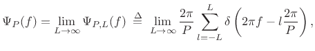 |
(B.54) |
show that a direct inverse-Fourier transform calculation gives
![$\displaystyle \psi_{P,L}(t) = \frac{\sin\left[\pi(2L+1)\frac{t}{P}\right]}{\sin\left( \pi \frac{t}{P}\right)},$](http://www.dsprelated.com/josimages_new/sasp2/img2521.png) |
(B.55) |
and verify that the peaks occur everyseconds and reach height
. Also show that the peak widths, measured between zero crossings, are
, so that the area under each peak is of order 1 in the limit as
. [Hint: The shift theorem for inverse Fourier transforms is
, and
.]
Next Section:
Poisson Summation Formula
Previous Section:
Sinc Impulse


