Practical Computation of the STFT
While the definition of the STFT in (7.1) is useful for
theoretical work, it is not really a specification of a practical
STFT. In practice, the STFT is computed as a succession of FFTs of
windowed data frames, where the window ``slides'' or ``hops'' forward
through time. We now derive such an implementation of the STFT from
its mathematical definition.
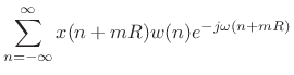
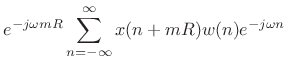
The STFT in (7.1) can be rewritten, adding  to
to  , as
, as
In this form, the data centered about time
are translated to time
0, multiplied by the (let's assume
zero-phase) window

, and then
the
DTFT is performed. Since the nonzero portion of the windowed data
is centered on time zero, the DTFT can be replaced by the
DFT (or
FFT). This effectively
samples the DTFT in frequency. This
sampling will not cause (time)
aliasing if the number of samples
around the unit circle is greater than the width (in samples) of the
time interval including all nonzero datapoints. In other words,
sampling the frequency axis is information-preserving when the
signal
is properly
time limited.
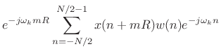
8.3Let

denote the window length (typically an
odd number) and

be the DFT length (typically a power of 2). Then
sampling (
7.3) at
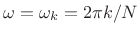
,
, and using the fact that the window

is
time-limited to less than

samples centered about time zero, yields
Since indexing in the DFT is modulo
, the sum over
can be
``rotated'' to a sum from 0 to

as is conventionally implemented
for the DFT. In practice, this means that the right half of the
windowed data frame goes at the beginning of the FFT input buffer, and
the left half of the windowed frame goes at the end, with
zero-padding
in the middle (see Fig.
2.6b on page
![[*]](../icons/crossref.png)
for
an illustration).
Next Section: Summary of STFT Computation Using FFTsPrevious Section: Mathematical Definition of the STFT