STFT Filter Bank

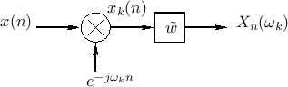
Free Books Spectral Audio Signal Processing

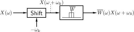
Each channel of an STFT filter bank implements the processing shown in Fig.9.4. The same processing is shown in the frequency domain in Fig.9.5. Note that the window transform $W(\omega)$ is complex-conjugated because the window is flipped in the time domain, i.e., $w(-n)\;\leftrightarrow\;\overline{W(\omega)}$ when is real [264].

**Figure:** One channel of the STFT filter bank computing **$X_n(\omega_k)=(x_k\ast \protect{\tilde w})(n)$** , where **$x_k(n)\isdeftext x(n)\exp(-j\omega_k n)$** , and **$\protect{\tilde w}\protect\isdeftext \protect\hbox{\sc Flip}(w)$** .
$\includegraphics{eps/fbs-chan}$

**Figure:** One channel of the STFT filter bank in the frequency domain ( **$\overline {W}$** denotes the complex conjugate of ).
$\includegraphics{eps/fbs-chan-fd}$

These channels are then arranged in parallel to form a filter bank, as shown in Fig.9.3. In practice, we need to know under what conditions the channel filters will yield perfect reconstruction when the channel signals are remodulated and summed. (A sufficient condition for the sliding STFT is that the channel frequency responses overlap-add to a constant over the unit circle in the frequency domain.) Furthermore, since the channel signals are heavily oversampled, particularly when the chosen window has low side-lobe levels, we would like to be able to downsample the channel signals without loss of information. It is indeed possible to downsample the channel signals while retaining the perfect reconstruction property, as we will see in §9.8.1.

Computational Examples in Matlab

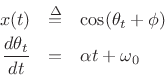
In this section, we will take a look at some STFT filter-bank output signals when the input signal is a ``chirp.'' A chirp signal is generally defined as a sinusoid having a linearly changing frequency over time:

$\begin{eqnarray*} x(t) &\isdef & \cos(\theta_t+\phi)\\ \frac{d\theta_t}{dt} &=& \alpha t + \omega_0 \end{eqnarray*}$

The matlab code is as follows:

N=10;           % number of filters = DFT length
fs=1000;        % sampling frequency (arbitrary)
D=1;            % duration in seconds

L = ceil(fs*D)+1; % signal duration (samples)
n = 0:L-1;        % discrete-time axis (samples)
t = n/fs;         % discrete-time axis (sec)
x = chirp(t,0,D,fs/2);   % sine sweep from 0 Hz to fs/2 Hz
%x = echirp(t,0,D,fs/2); % for complex "analytic" chirp
x = x(1:L);       % trim trailing zeros at end
h = ones(1,N);    % Simple DFT lowpass = rectangular window
%h = hamming(N);  % Better DFT lowpass = Hamming window
X = zeros(N,L);   % X will be the filter bank output
for k=1:N         % Loop over channels
  wk = 2*pi*(k-1)/N;
  xk = exp(-j*wk*n).* x;  % Modulation by complex exponential
  X(k,:) = filter(h,1,xk);
end

Figure 9.6 shows the input and output-signal real parts for a ten-channel DFT filter bank based on the rectangular window as derived above. The imaginary parts of the channel-filter output signals are similar so they're not shown. Notice how the amplitude envelope in each channel follows closely the amplitude response of the running-sum lowpass filter. This is more clearly seen when the absolute values of the output signals are viewed, as shown in Fig.9.7.

**Figure 9.6:** 10-Channel DFT filter bank real-chirp response. Output real part versus time in each channel (rectangular window).
$\includegraphics[width=\twidth,height=6.5in]{eps/dcrrrp}$

**Figure 9.7:** 10-Channel DFT filter bank real-chirp response. Output magnitude versus time in each channel (rectangular window).
$\includegraphics[width=\twidth,height=6.5in]{eps/dcrr}$

Replacing the rectangular window with the Hamming window gives much improved channel isolation at the cost of doubling the channel bandwidth, as shown in Fig.9.8. Now the window-transform side lobes (lowpass filter stop-band response) are not really visible to the eye. The intense ``beating'' near dc and half the sampling rate is caused by the fact that we used a real chirp. The matlab for this chirp boils down to the following:

function x = chirp(t,f0,t1,f1);
beta = (f1-f0)./t1;
x = cos(2*pi * ( 0.5* beta .* (t.^2) + f0*t));

We can replace this real chirp with a complex ``analytic'' chirp by replacing the last line above by the following:

x = exp(j*(2*pi * ( 0.5* beta .* (t.^2) + f0*t)));

Since the analytic chirp does not contain a negative-frequency component which beats with the positive-frequency component, we obtain the cleaner looking output moduli shown in Fig.9.9.

Since our chirp frequency goes from zero to half the sampling rate, we are no longer exciting the negative-frequency channels. (To fully traverse the frequency axis with a complex chirp, we would need to sweep it from $-\pi$ to $\pi$ .) We see in Fig.9.9 that there is indeed relatively little response in the ``negative-frequency channels'' for which , but there is some noticeable ``leakage'' from channel 0 into channel , and channel 5 similarly leaks into channel 6. Since the channel pass-bands overlap approximately 75%, this is not unexpected. The automatic vertical scaling in the channel 7 and 8 plots shows clearly the side-lobe structure of the Hamming window. Finally, notice also that the length start-up transient is visible in each channel output just after time 0.