Some Thoughts on Sampling

Some time ago, I came across an interesting problem. In the explanation of sampling process, a representation of impulse sampling shown in Figure 1 below is illustrated in almost every textbook on DSP and communications. The question is: how is it possible that during sampling, the frequency axis gets scaled by $1/T_s$ -- a very large number? For an ADC operating at 10 MHz for example, the amplitude of the desired spectrum and spectral replicas is $10^7$! I thought that there must be something wrong somewhere.

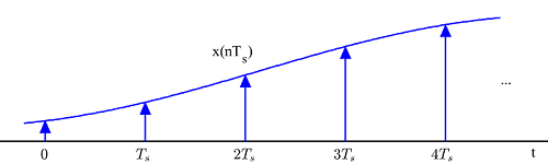
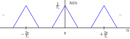
Figure 1: Sampling in time domain creates spectral replicas in frequency domain, each of which gets scaled by $1/T_s$

I asked a few DSP experts this question. They did not know the answer as well. Slowly I started to understand the reason why it is true, and in fact, makes perfect sense. The answer is quite straightforward but I did not realize it immediately. Since this is a blog post, I can take the liberty of explaining the route I took for this simple revelation.

A Unit Impulse

---

My first impression was that whenever impulses are involved, everything that branches from there becomes fictitious as well. A continuous-time unit impulse is defined as shown in Figure 2.

Area under a rectangle = $\Delta \cdot \frac{1}{\Delta} = 1$, or $\int \limits_{-\infty} ^{+\infty} \delta (t) dt = 1$

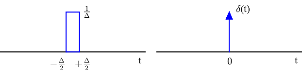
Figure 2: Definition of a unit impulse

Clearly, the sampling scale factor is independent of how we define a unit impulse and its infinite height. The next step might be to look into a sequence of unit impulses: an impulse train.

An Impulse Train

---

An impulse train is a sequence of impulses with period $T_s$ defined as
    $$        p(t) = \sum \limits _{n=-\infty} ^{+\infty} \delta (t-nT_s) $$
The standard method to derive its Fourier Transform is through expressing the above periodic signal as a Fourier series and then finding Fourier series coefficients as follows.
First, remember that a signal $x(t)$ with period $T_s$ can be expressed as

$$x(t) = \sum \limits _{k=-\infty} ^{+\infty} x_k e^{jk \Omega_s t}$$ where $\Omega_s = 2\pi/T_s$ and it can be seen as the fundamental harmonic in the sequence of frequencies $k\Omega_s$ with $k$ ranging from $-\infty$ to $+\infty$. Here, $x_k$ are the Fourier series coefficients given as

$$     x_k = \frac{1}{T_s} \int _{-T_s/2} ^{T_s/2} x(t) e^{-jk \Omega_s t} dt$$ 

When $p(t)$ is an impulse train, one period between $-T_s/2$ and $+T_s/2$ only contains a single impulse $\delta (t)$. Thus, $p_k$ can be found to be

$$       p_k = \frac{1}{T_s} \int _{-T_s/2} ^{T_s/2} \delta (t) e^{-jk \Omega_s t} dt = \frac{1}{T_s} \cdot e^{-jk \Omega_s \ \cdot \ 0}= \frac{1}{T_s}$$

Plugging this in definition above and using the fact that $\mathcal{F}\left\{e^{jk \Omega_s t}\right\} = 2\pi \delta \left(\Omega - k\Omega_s \right)$ and $\Omega_s = 2\pi/T_s$, we get

$$    P(\Omega) = \frac{1}{T_s} \sum \limits _{k=-\infty} ^{+\infty} \mathcal{F}\left\{ e^{jk \Omega_s t}\right\} = \frac{2\pi}{T_s} \sum \limits _{k=-\infty} ^{+\infty} \delta \left( \Omega - k \frac{2\pi}{T_s}\right)$$

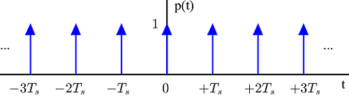
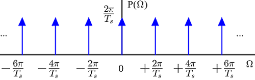
Figure 3: Fourier Transform of an impulse train in time domain is another impulse train in frequency domain

The resulting time and frequency domain sequences are drawn in Figure 3 above which is a standard figure in DSP literature. However, it really comes as a surprise that an impulse train has a Fourier Transform as another impulse train, although the Fourier Transform of a unit impulse is a constant. What happened to the concept that a signal narrow in time domain has a wide spectral representation? Going through this method, it is not immediately clear why.

So I thought of deriving it through some other technique. Note that I prefer to use the frequency variable $F$ instead of $\Omega$.

$$\int _{-\infty} ^{+\infty} \sum _{n=-\infty} ^{+\infty} \delta(t - nT_s) e^{-j2\pi F t} dt = \sum _{n=-\infty} ^{+\infty} \int _{-\infty} ^{+\infty} \delta(t - nT_s) e^{-j2\pi F t} dt $$

$$= \sum _{n=-\infty} ^{+\infty} e^{-j2\pi F nT_s}$$

From here, there are many techniques to prove the final expression, and the mathematics becomes quite cumbersome. So I just take the route of visualizing it and see where it leads.

Where the Impulses Come From

---

First, the Fourier Transform of a time domain impulse train can be seen as the sum of frequency domain complex sinusoids with ``frequencies'' equal to $nT_s$, or periods equal to $\frac{1}{nT_s} = \frac{F_s}{n}$. Furthermore, the above signal is periodic with period of first harmonic $1/T_s=F_s$.

$$  \sum _{n=-\infty} ^{+\infty} e^{-j2\pi (F+F_s)   nT_s} = \sum _{n=-\infty} ^{+\infty} e^{-j2\pi F   nT_s}\cdot \underbrace{e^{-j2\pi n}}_{1} = \sum _{n=-\infty} ^{+\infty} e^{-j2\pi F   nT_s}$$

Therefore, for the sake of better visualization, we limit ourselves to the range $[0,F_s)$ when drawing the figures in frequency domain. Whatever happens here gets repeated elsewhere. Figure 4 illustrates 3 frequency domain complex sinusoids $e^{-j2\pi F   nT_s}$ for $n=1,2$ and $3$, with frequencies $T_s, 2T_s$ and $3T_s$, respectively. Note how within a period of $F_s$, the first completes one cycle, while the other two complete two and three cycles, respectively. Here, we deliberately refrained from drawing the result for $n=0$ which is a straight line at $1$ on $I$ axis.  

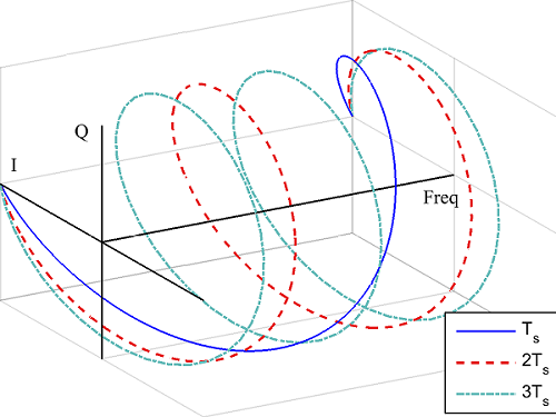
Figure 4: 3 frequency domain complex sinusoids $e^{-j2\pi F   nT_s}$ for $n=1,2$ and $3$, with frequencies $T_s, 2T_s$ and $3T_s$, respectively, in the range $[0,F_s)$

For a closer look, see the signal decomposed into $I$ and $Q$ axes. Clearly, the $I$ axis consists of $\cos (2\pi F   nT_s)$ and the $Q$ axis consists of $-\sin(2\pi F   nT_s)$ again with $n = 1,2$ and $3$. This is shown in Figure 5.

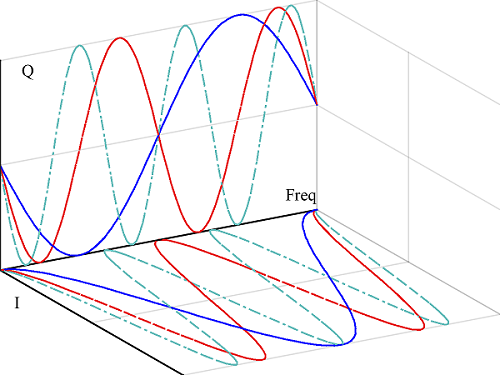
Figure 5: $I$ and $Q$ decomposition of Figure 4. The $I$ axis consists of $\cos (2\pi F   nT_s)$ and the $Q$ axis consists of $-\sin(2\pi F   nT_s)$ again with $n = 1,2$ and $3$, in the range $[0,F_s)$

Having understood the basic concept, we now divide the range $[0,F_s)$ into $N$ segments each with width $\nu$.
    \begin{equation*}
       \nu  = \frac{F_s}{N}
    \end{equation*}
This implies that for integer $k$,
    \begin{equation*}
        F \approx k\nu = k \frac{F_s}{N}, \qquad fT_s = \frac{k}{N}
    \end{equation*}

The result of summing the sinusoids shown in Figure 5 for a large $N$ is drawn in Figure 6.

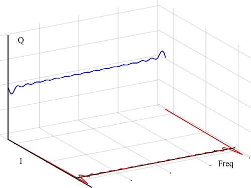
Figure 6: Summing the $I$ and $Q$ parts from Figure 5 but for a very large $N$ in the range $[0,F_s)$. The $Q$ part is seen converging to 0 while the $I$ part approaches an impulse, half of which is visible at $0$ and half at $F_s$

The rectangle at $k=0$ has a height of $N$ since it is a sum of $1$ for all $N$ values of $n$. It can now be concluded that

• $I$ arm -- the expression $\sum _{n=-\infty} ^{+\infty} \cos(2\pi nk/N)$ -- approaches $N$ at $k=0$ in each period $[0,F_s)$. As $\nu \rightarrow 0$, $N \rightarrow \infty$ and it becomes an impulse (strictly speaking, the limit does not exist as a function and is rather known as a ``distribution'').
• On the other hand, the $Q$ arm  -- the expression $\sum _{n=-\infty} ^{+\infty} -\sin(2\pi n k/N)$ -- vanishes.

    
The scaling factor here can be found again by taking the area under the first rectangle. Thus,  
      

Area under the rectangle $= N \cdot \nu = N \cdot \frac{F_s}{N} = F_s,$   

the same as found in Figure 3 (except the factor of $2\pi$). Since it is a periodic signal, it consists of impulses repeating at integer multiples of $F_s$ -- just what we saw in Figure 3 (except the $2\pi$ factor as we are dealing in $F$ now). The complete sequence is now drawn in Figure 7.

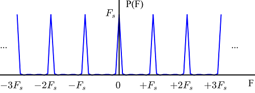
Figure 7: Displaying the $I$ branch from Figure 6 in the range $(-3F_s,+3F_s)$ for large $N$

It was then I realized my problem. All the graphs and curves I have drawn, and DSP textbooks draw for that matter, use the wrong scaling on the axes! Although the time and frequency domain impulse sequences look pretty much similar to each other, they are not. Imagine a very large number, say $L$. Now if I draw the time and frequency domain representations of an impulse train within the range $-L$ to $+L$, the signals would look like as illustrated in Figure 8 for a sample rate of $10$ MHz. As it is evident, all the confusion in the y-axis was due to incorrect scaling at the x-axis!   

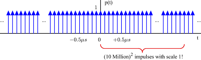
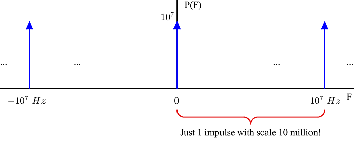
Figure 8: For a $10$ MHz sample rate, there are (10 million)$^2$ impulses in time domain for just 1 in frequency domain

Here, it is easier to recognize that for an ADC operating at 10 MHz, there are (10 million)$^2$ impulses on the time axis, for just one such impulse on the frequency axis. Let us express the equivalence of energy in time and frequency domains (known as Parseval's relation) in a different way.
    \begin{equation*}
        \lim_{L \to \infty} \int \limits _{-L}^{+L} |x(t)|^2 dt = \lim_{L \to \infty} \int \limits _{-L}^{+L} |X(F)|^2 df
    \end{equation*}Clearly, the scaling of the frequency axis by $F_s$ seems perfectly logical. A signal narrow in time domain is wide in frequency domain, finally! I must say that this is the same figure as Figure 3 but until I went this route, I did not figure (pun intended) this out.

This reminded me of drawing the structure of an atom along with the solar system to indicate some similarity, without mentioning their respective scales, as in Figure 9.

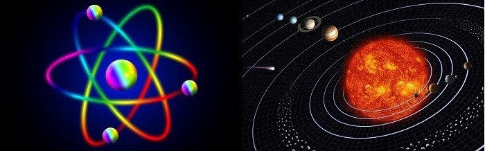
Figure 9: An atom and solar system

This also reinforced my concept of using the frequency variable $F$ instead of $\Omega$. While $\Omega$ has its advantages at places, the variable $F$ connects us with what is out there: the reality. The commonly used ISM band is $2.4$ GHz, not $4.8\pi$ G-radians/second.

Going into Discrete Domain

---

Let us turn our thoughts in discrete domain now. There are two points to consider in this context.

1. The main difference between a continuous-time impulse and a discrete-time impulse is that a discrete-time impulse actually has an amplitude of unity; there is no need to define the concept related to the area under the curve.
2. There is a factor of $N$ that gets injected into expressions due to the way we define Fourier Transforms. This is the equivalent of the factor $2\pi$ for continuous frequency domain $\omega$ in Discrete-Time Fourier Transform (DTFT).

      \begin{equation*}
        x[n] = \frac{1}{2\pi} \int \limits _{\omega=-\pi} ^{+\pi} X(e^{j\omega})\cdot e^{j\omega n} d \omega, \qquad x[n] = \frac{1}{N} \sum \limits_{k=-N/2}^{+N/2-1} X[k]\cdot e^{j2\pi \frac{k}{N}n}
      \end{equation*}

A discrete impulse train $p[n]$ is a sequence of unit impulses repeating with a period $M$ within our observation window (and owing to DFT input periodicity, outside the observation window as well). Figure 10 illustrates it in time domain for $N=15$ and $M=3$.
 

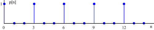
Figure 10: Discrete impulse train in time domain for $N=15$ and $M=3$

To compute its $N$-point DFT $P[k]$,
    \begin{align*}
         P[k] =& \sum \limits _{n=0} ^{N-1} p[n] e^{-j2\pi\frac{k}{N}n} = \sum \limits _{m=0} ^{N/M-1} 1 \cdot e^{-j2\pi\frac{k}{N/M}m} \\
              =& \begin{cases}
                    \frac{1}{M}\cdot N   &  k = integer \cdot \frac{N}{M} \\
                    0  & elsewhere
                \end{cases}
    \end{align*}A few things to note in this derivation are as follows.

• I write DFT emphasizing on the expression $\frac{k}{N}$ because it corresponds to the continuous-time frequency $\frac{F}{F_s}$, explicitly exposing $n$ as the time variable similar to its counterpart $t$ (think of $2\pi \frac{F}{F_s}n$, or $2\pi ft$).
• From going to second equation from the first, I use the fact that $p[n]=0$ except where $n=mM$.
• The third equation can be derived, again, in many ways such as the one described in the continuous-time case described before.

The final DFT output is shown in Figure 11 for $N=15$ and $M=3$.
 

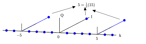
Figure 11: Discrete impulse train in frequency domain for $N=15$ and $M=3$

Note how impulse train in time domain is an impulse train in frequency domain. So for $N=15$ and a discrete-time impulse train with a period of $3$, the DFT is also an impulse train with a period of $N/3 =5$. Moreover, the unit impulses in frequency domain have an amplitude of $N/3=5$ as well. Observe that a shorter period $M$ in time domain results in a longer period $N/M$ in frequency domain. Also, the amplitude of those frequency domain impulses is $N/M$ times larger as well: compare with $2\pi/T_s$ in Figure 3.

This is the same result as in continuous frequency domain with impulse train having a period of $F_s$ as well as a scaling factor of $F_s$. However, it is much clearer to recognize in discrete domain due to the finite DFT size $N$. That is why I talked about limiting the continuous frequency range within $\pm L$ for a large $L$ and wrote Parseval's relation as above.

Sampling in Discrete Domain: Downsampling

---

With the above findings, we want to see what happens when a discrete-time signal is sampled with a discrete-time impulse train. In DSP terminology, this process is known as downsampling. Although it is common to discuss downsampling as a separate topic from sampling a continuous-time signal, both processes are intimately related and offer valuable insights into one another.

A signal $x[n]$ can be downsampled by a factor of $D$ by retaining every $D$th sample and discarding the remaining samples. Such a process can be imagined as multiplying $x[n]$ with an impulse train $p[n]$ of period $D$ and then throwing off the intermediate zero samples (in practice, no such multiplication occurs as zero valued samples are to be discarded). As a result, there is a convolution between $X[k]$ and $P[k]$ and $D$ spectral copies of $X[k]$ arise: one at frequency bin $k=0$ and others at $\pm integer \cdot N/D$, all having a spectral amplitude of $N/D$. As $D$ increases, the spectral replicas come closer and their amplitudes decrease proportionally. This is illustrated in Figure 12 for downsampling a signal by $D=3$.

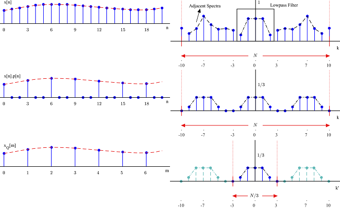
Figure 12: Downsampling a signal $x[n]$ by $D=3$ in time and frequency domains

This is the same concept as sampling a continuous-time signal. Just as we decrease the amplitudes and spread of the resulting spectral copies by reducing the sampling rate, we decrease the amplitudes and spread of the resulting spectral copies by throwing off more samples, i.e., reducing the sampling rate. In the former, this happens in proportion to $1/T_s$; in the latter, in proportion to $1/D$.

Put in this way, $1/D$ is choosing $1$ out of every $D$ samples. And $1/T_s$ is choosing $1$ out of every $T_s$ samples if there ever were. In this context, $1/T_s$ is the probability density function (pdf) of a uniform random variable in the range $[0,T_s)$.

An Alternative View

---

Carrying on, now we can look into an alternative view on sampling. First, consider the scaling property of the Fourier Transform.
    \begin{equation*}
        x(a\cdot t) \quad \xrightarrow{{\mathcal{F}}} \quad \frac{1}{|a|} X\left(\frac{F}{a} \right)
    \end{equation*}
Second, instead of impulse sampling, we can just see it as a scaling of the time axis. Taking the constant $a$ as $T_s$,
    \begin{equation*}
        x(T_s \cdot t) = x(tT_s) \quad \xrightarrow{{\mathcal{F}}} \quad \frac{1}{T_s} X\left(F = \frac{f}{T_s} \right)
    \end{equation*}
Here, $x(tT_S)$ is the counterpart of $x(nT_s)$ from impulse sampling with the difference being a real number $t$ instead of an integer $n$. Also, instead of nano and micro seconds, $T_s$ has no units and we just deal it in the limiting case where the interval $[0,T_s)$ is divided into infinitesimally small segments and $T_s$ is just a positive number. In this way, this case becomes similar to downsampling where $D$ is always greater than $1$.

The spectrum x-axis also gets scaled by $T_s$ leading to the fundamental relationship between continuous-time frequency $F$ and discrete-time frequency $f$.
    \begin{equation*}
        f = F\cdot T_s \qquad \rightarrow \qquad \omega = \Omega \cdot T_s
    \end{equation*}Within this framework, it is only after discarding the intermediate ``samples'' that the spectral replicas emerge. This is a result of defining the frequency axis in relation to periodic signals. There might be an alternative definition of frequency that would make processing the samples easier.

Sign in