


Radio Frequency Distortion Part II: A power spectrum model
Summary
This article presents a ready-to-use model for nonlinear distortion caused by radio frequenfcy components in wireless receivers and linear transmitters.
Compared to the similar model presented in my earlier blog entry, it operates on expectation values of the the power spectrum instead of the signal itself: Use the signal-based model to generate distortion on a signal, and the one from this article to directly obtain the power spectrum much more efficiently.
In communications systems design, the previous one might be referred to as link-level simulator model, whereas one presented here is a system-level simulator model.
Besides simulation, it can be a useful tool for other applications, whereever there is need to predict unwanted emissions. For example, future power-saving algorithms could adaptively back off the amplifier, based on a prediction of unwanted emissions and possibly time-changing emission limits.
This article discusses the model, compares to a baseband-equivalent model and provides both simple example code and an efficient implementation based on FFT that uses only real-valued arithmetics.
Introduction
Radio frequency components in mobile wireless devices and basestations cause distortion on both transmitted and received signals. Distortion deteriorates the quality of the radio link passing through the component, and also causes interference to other links via unwanted emissions.
While my earlier blog entry discusses distortion modeling on a complex baseband-equivalent signal, this is not practical when modeling whole communications systems.
Motivation
Distortion is unfortunately a major issue for wireless links and systems, because the technology used for analog radio frequency electronics has not evolved at the same mind-boggling rate as digital signal processing. And even worse, cost pressure often forces implementation of analog radio frequency circuitry on a digital-optimized CMOS semiconductor process with all its inherent problems, not the least of them the immense cost of design iterations.
Modeling distortions is essential during the design phase, and possibly also for future devices that act more "intelligently" to meet regulators' spectral emission mask constraints with a cost-efficient radio.
Frequently, the term link level simulator is used for a model of a single wireless link that operates on sampled baseband signals. A system level simulator considers more than one link at the same time, but uses by necessity a more abstract representation of each link.
For example in cellular radio, one basestation often serves dozens of mobile devices. To get meaningful data on interference between cells and their impact to bit error rate and outage probability, many basestations need to be included, resulting in a hundred or more links simulated simultaneously.
Clearly, the distortion model needs to be efficient: During the course of a simulation, it may be executed millions of times.
Modeling of distortion is also important for novel radio concepts that are under research, where nodes are aware of the interference they are causing to others ("Interference-aware scheduling", "Cognitive Radio", "Whitespaces" etc):
For example, a distortion model can predict the unwanted emissions based on the frequency ranges allocated for transmission and the known spectral power density, allowing a transmitter to adapt its transmissions [2].
Transmitter and receiver distortion
In a transmitter, the power amplifier is the most important source of distortion, because the signal is processed at a high power level.
For a receiver, the low-noise amplifier and mixer tend to be the most critical, because it is difficult or impossible to filter out interfering signals before those stages.The main challenge for receivers is to deal with signals that are not under the control of the device.
For example, a receiver suffers from intermodulation, where two interfering signals cause distortion products at a completely different frequency. A somewhat related problem is crossmodulation, where a modulated signal at an arbitrary frequency is "picked up" by a strong, narrow-band interferer such as a GSM cellular phone.
Especially the distortion products at a receiver can be challenging to model, when large numbers of nodes are involved, because each transmitter's signal can potentially intermodulate with the signal of any other transmitter.
The presented model accurately reflects this behavior, for the price of a small-ish FFT/IFFT pair.
Power spectrum model example
A model using complex baseband-equivalent signals is impractical when only the distortion spectrum is of interest.
Therefore, an alternative model is proposed that directly operates on expectation values of the power spectrum instead of signal samples.
The signal is abstracted to a vector of power-vs-frequency values.
For example, in a LTE radio system, one might use
- One power value per subcarrier
- One power value for a group of 12 subcarriers spanning 180 kHz.
- One power value for a 5 MHz band
The best granularity depends on the purpose of the model: The price for higher accuracy is an increased computational effort.
As an example, consider a receiver with an interfering signal s1 and a wanted signal s2 picked up by the antenna. Both are 2 MHz wide. The spectrum is divided into 1 MHz subbands.
The signals could be modeled as follows:
s1=[0 0 4 4 0 0 0 0]
s2=[0 0 0 0 1 1 0 0]
Each number reflects a power value in its subband. Comparing the total power of both signals (all bins added), the level of s1 relative to s2 is 10 log10 (4+4)/(1+1) = 6 dB.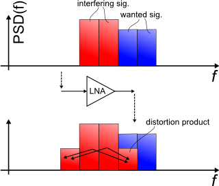
Figure 1: Received signal at a receiver's low-noise amplifier (LNA)
Figure 1 illustrates the power spectral density (PSD) of the signal at the input and output of the receiver. The two strong subbands of the interfering signal cause an intermodulation product that overlaps one subband of the wanted signal and deteriorates its signal-to-noise ratio.
The wanted signal also causes intermodulation products with itself and the interfering signal. Those products are omitted in the picture but correctly predicted by the model.
Reference power
The power levels in s1 and s2 can be referred to an arbitrary value, but the model needs to be calibrated accordingly. For example, one could define powers in units of Watts. Under this convention, a received signal of -20 dBm=10 microwatts corresponds to a number of 10-5 in a single bin. Alternatively, the same power might be distributed over for example 10 different bins, with a value of 10-6 in each bin.
The reference power "1" is chosen arbitrarily, but it relates to the "calibration" of the amplifier model.
Distortion process
Part I of this blog describes the distortion mechanisms that cause unwanted products at different frequencies.
In the presented model, the signal representation is different, namely a vector of power values instead of a complex baseband-equivalent siganl. Otherwise, exactly the same mechanics apply.
The key to this model is equation (16) in [1]: It states that the power spectrum of a polynomial bandpass nonlinearity can be calculated by repeatedly convolving the continuous power spectrum of the input signal with itself, and a frequency-reversed replica.
The 3rd order distortion product follows as
Sdist3(f)=a3 S(f) S(f)S(-f) S(f)S(-f) |
(1) |
where S(f) is the input spectrum, S(-f) a frequency-mirrored replica and Sdist3(f) the output spectrum of a pure 3rd-order nonlinearity. The star "" denotes convolution, and a3 is a constant.
Using a frequency-discrete signal, for example the sum of LNA input signal from the earlier example sin=s1+s2 (vectors in boldface) the output vector of the 3rd order distortion product can be calculated directly:
| sdist3=conv(conv(sin, sin), fliplr(sin)) | (2) |
Using Matlab notation, conv(...) performs discrete convolution, and fliplr(...) results in the mirror image of a vector.
sdist3 is the pure distortion term, whereas an amplifier naturally also amplifies the input signal. To obtain the full output signal, add a scaled version of the input signal. Often, amplifier models are normalized to unity gain. If so, a1 equals 1.
| sout=a1 sin+a3 sdist3. | (3) |
Direct implementation in Matlab
Below follows a short Matlab program (download) that implements eq. (2) and (3):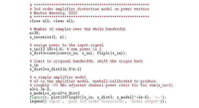
Figure 2: Matlab implementation of EQ(EQ)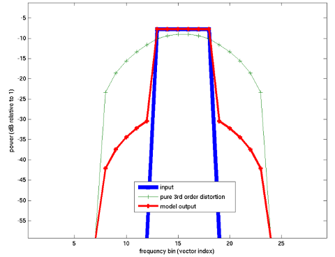
Figure 3: Output spectrum from the program in Figure 2
blue: input signal
green: pure distortion
red: amplifier model
Running the same program with a higher number of samples (download) results in the following spectrum:
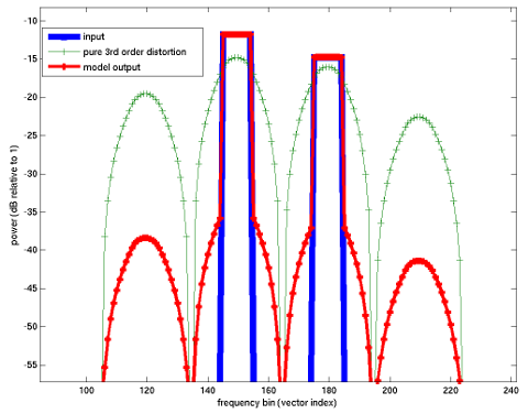
Figure 4: Output spectrum of a more complex signal
Efficient implementation
The model has a small flaw: It requires two convolutions, which can become impractical to compute:
A system level simulation may execute the model for every transmitter and every receiver at every time step, easily resulting in tens of millions of model evaluations. Computational efficiency becomes a concern.
Fortunately, FFT comes to our help not only once but twice:
a) Convolution can be performed efficiently using an FFT-IFFT pair
b) A double convolution can use the same FFT-IFFT pair.
For a third-order model, the bandwidth of distortion products can be up to three times the original bandwidth.
Therefore, we need to zero-pad the power vectors to a sufficient width - at least three times the width of the original signal (minus one, to be accurate). Zero-padding to an arbitrary width is allowed, and powers of two tend to be most "FFT-friendly".
After zero-padding, we can implement the convolution via FFT:
| conv(a, a) =ifft(fft(a) .* fft(a)) | (4) |
The ".*"-operator performs an element-by-element multiplication between vectors.
Reversing a vector is equivalent to taking the complex conjugate after IFFT. Thus, the original 3rd-order distortion model can be rewritten as
| conv(conv(a, a), fliplr(a))=ifft(fft(a) .* fft(a) .* conj(fft(a)) | (5) |
Further, we can expand the complex multiplication to allow an implementation with real-valued arithmetics:
| real + i imag := fft(a) conv(conv(a, a), fliplr(a)) = ifft((real+i imag) .* (real .^ 2 + imag .^ 2)). |
(6) |
Here (download) is a matlab example that implements eq. (4) to (6).
Implications
For a polynomial nonlinearity and input signals with a Gaussian amplitude pdf, the model gives a correct estimate of the distortion spectrum.
However, what we should keep in mind is that the model operates on samples of a continuous power spectrum S(f). Each sample represents the area under a piece of S(f) as a discrete Dirac-pulse sample with an infinitesimally narrow bandwidth.
The difference can be important, mainly when dealing with strong narrowband signals that fit into a single bin:
For a modulated signal, the nth order distortion products occupy n times the original bandwidth. However, since the Dirac-pulse sample has zero bandwidth, this property is lost in the sampled spectrum.
For example:
- a 180 kHz wide resource block creates intermodulation products with itself into the adjacent lower and upper resource block, each having a 180 kHz bandwidth.
- A 180 kHz wide resource block represented by a single sample does not create intermodulation products into the adjacent samples.
A straightforward solution is to sub-divide the smallest bandwidth of interest into three or more pieces, such as three times 60 kHz. However, in many applications, narrowband signals are unlikely or impossible, and the inaccuracy does not matter. The example below show that one sample per subband can be very accurate.
A Gaussian amplitude pdf is approximated well by OFDM signals, but somewhat less so by for example single-carrier FDMA (SC-FDMA). This is to be expected, since the main reason for SC-FDMA over OFDM is to avoid the Gaussian pdf and its long tails, leading to lower distortion at the same power.
Implementation and accuracy
A small, self-contained Matlab simulator was used to model and compare distortion products of a complex-baseband model and a power spectrum model.
Both implement a 3rd order polynomial nonlinearity that is an accurate model for weakly nonlinear circuits. The OFDM signal in the baseband part approximates a Gaussian amplitude pdf, which is assumed in the power spectrum part.
When using a sufficient number of spectrum samples, the results are practically identical, but the computational effort for the latter calculation is orders of magnitude lower.
Note that the model was calibrated "by eye". Equations to convert the parameters between both types of models can be found in [1].
The following plots shows the simulated signal spectra resulting from both models.
Note that I'm drawing the spectrum as a series of horizontal lines to illustrate the bandwidth of each bin, although Dirac-like pulses would be more accurate.
Limitations for narrow-band signals
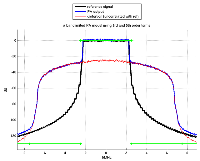
Figure 5: Comparison of models on a single-subband signal, using one sample per subband
black: The input signal: OFDM with raised-cosine windowing
blue: The output signal of the baseband-equivalent model
red: The isolated distortion term of the baseband-equivalent model, which is uncorrelated with the input signal
green: The output of the power-spectrum model presented in this article.
In Figure 5, the full transmit power is concentrated into a single transmit subband, from -2.25 to 2.25 MHz.
The power spectrum model uses only one subdivision per transmit subband.
The discussed limitation of the power spectrum model (green) is clearly visible: It does not create intermodulation products into adjacent bands.
A straightforward solution is to use more samples per subband: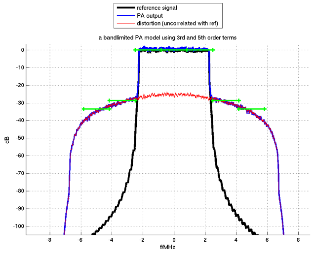
Figure 6: Comparison of models, single-subband signal and three samples per subband
In Figure 6, the green lines approximate the out-of-band emissions quite accurately.
The cases in Figures 5 and 6 are presented to show the limitations of the model, but they are not too relevant in many practical applications: Usually we are less interested in the interaction of a signal with itself - there are easier ways to get that information. The real challenge arises when faced with a large number of signals and the resulting combinatorial explosion of possible interactions.
Examples using wider-band signals
As soon as the power is distributed over several resources, granularity becomes less of a concern. The following simulation result distributes the power over seven subbands, using three blocks with 1/1/5 subbands in each..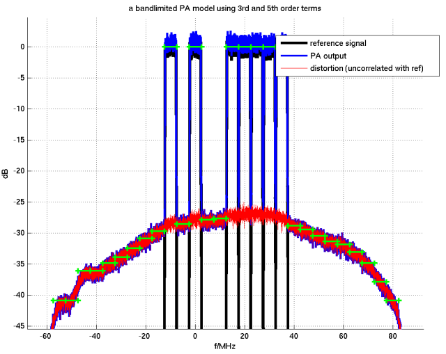
Figure 7: comparison of models for a more complex signal
Comparing the green curve (power spectrum model) and the blue or red curve (complex baseband model) it is clear to see that the power spectrum model gives the same result, even though the efford for its computation is orders of magnitude smaller.
The granularity can be further reduced using for example three spectrum samples per subband, improving the resolution at the spectrum edges somewhat. An even finer granularity, possibly down to subcarrier level, can be convenient to accurately model the effects of guard bands. 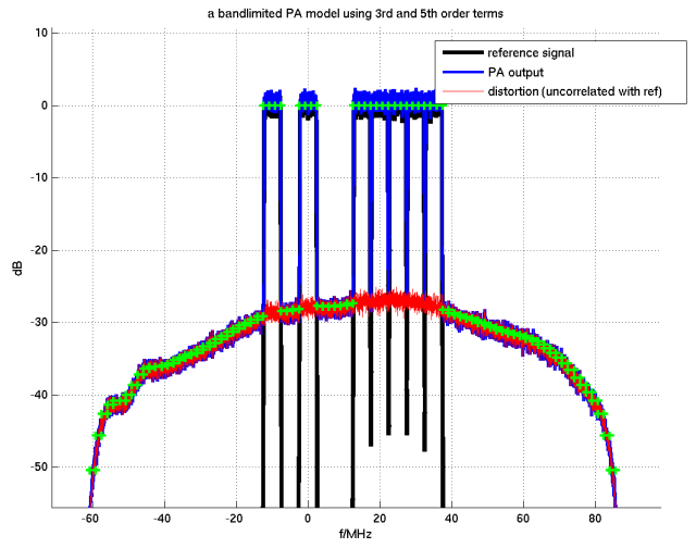
Figure 8: Each subband further divided into three parts
Conclusion
The article presents a model for weakly nonlinear distortion, as is typical in wireless applications. The model operates on the power spectrum of a signal. It is based on the derivation from [1].
For signals that approximate a Gaussian amplitude pdf (such as OFDM), and a sufficient density of spectrum samples, the result is practically identical to that of a baseband model.
A computationally highly efficient example implementation is presented.
Links
- Understanding Distortion part I: My earlier blog entry.
- A straightforward implementation in Matlab: download.
- Matlab example for convolution via FFT/IFFT: download
- The simulator used for Figures 5-8: download.
References
[1] G. Zhou and R. Raich, “Spectral analysis of polynomial nonlinearity with applications to RF power amplifiers,” EURASIP Journal on Applied Signal Processing, no. 12, pp. 1831–1840, 2004.
Link
[2] P. Jänis, V. Koivunen and M. Nentwig: "Optimizing spectral shape under general spectrum emission mask constraints," 20th IEEE International Symposium on Personal, Indoor and Mobile Radio Communications, 2009, pp. 107-111
- Comments
- Write a Comment Select to add a comment
To post reply to a comment, click on the 'reply' button attached to each comment. To post a new comment (not a reply to a comment) check out the 'Write a Comment' tab at the top of the comments.
Please login (on the right) if you already have an account on this platform.
Otherwise, please use this form to register (free) an join one of the largest online community for Electrical/Embedded/DSP/FPGA/ML engineers:


