


The Risk In Using Frequency Domain Curves To Evaluate Digital Integrator Performance
This blog shows the danger in evaluating the performance of a digital integration network based solely on its frequency response curve. If you plan on implementing a digital integrator in your signal processing work I recommend you continue reading this blog.
Background
Typically when DSP practitioners want to predict the accuracy performance of a digital integrator they compare how closely that integrator's frequency response matches the frequency response of an ideal integrator [1,2]. Traditionally the assumption is: The closer a particular integrator's frequency response matches the frequency response of an ideal integrator the more accurate will be that integrator.
Years ago I accepted this assumption but I now believe it is not justified and I support my claim with a number of counter-examples presented in this blog. Let's begin by examining the frequency response of a theoretically ideal digital integrator and a few popular digital integrators.
Digital Integrator Frequency Responses
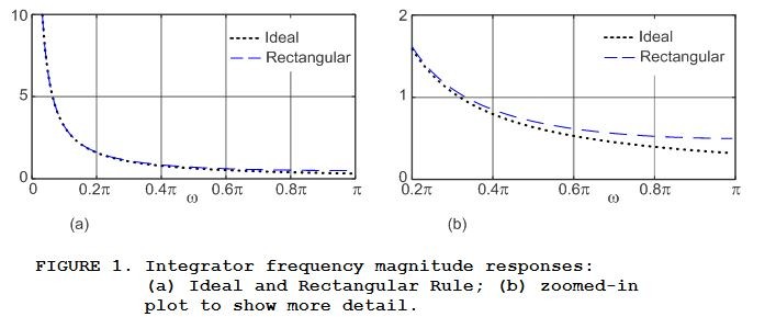
An ideal digital integrator has a frequency response described by:

where the frequency variable is $‑\pi ≤ \omega ≤ \pi$ measured in radians/sample. The positive-frequency ideal |HIdeal($\omega$)| magnitude response, shown as the dotted curves in Figure 1, is the response to which all digital integrator responses are compared. For example, the |HRect($\omega$)| frequency magnitude response of the Rectangular Rule integrator is also shown in Figure 1. Figure 1(b) shows the lower right side of Figure 1(a) in more detail.
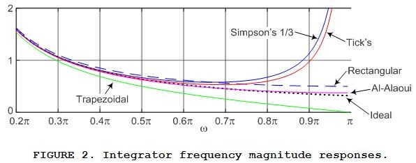
Characterizing other popular digital integrators, the frequency magnitude responses of the Rectangular Rule, Trapezoidal Rule, Simpson's 1/3 Rule, Tick's Rule, and what I call the "Al-Alaoui Method" digital integrators are shown in Figure 2. (I include the Al-Alaoui Method integrator here because it has gained some attention in recent years [3].) The difference equations and frequency response expressions for these five integrators are presented in Appendix A.
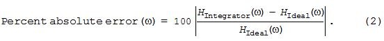
So, again, DSP practitioners typically assume the most accurate integrator is the one whose frequency response most closely matches the frequency response of an ideal integrator. To make such comparisons easier, Figure 3 shows the percent error, versus frequency, between the various integrators and an ideal integrator as computed by:
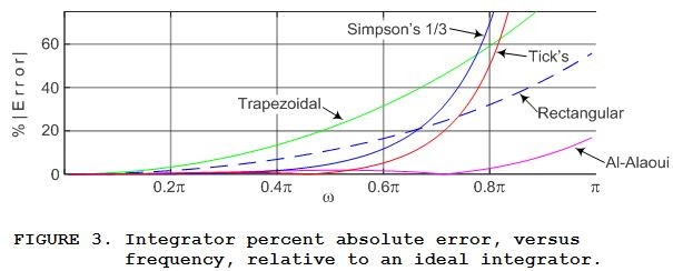
OK, examine Figure 3 carefully. That figure implies that if an integrator's input signal only contains spectral energy in the range of, say, 0 ≤ $\omega$ ≤ 0.65$\pi$ radians/sample then we should rank our five integrators' accuracy performances as shown in Table 1.
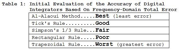
The Fallacy of Table 1
We might stop at this point and, based on Table 1, assume we have a reliable grasp on the relative accuracy performance of various popular digital integrators. But to do so would put us on a train bound for Failure City.
I support that last statement with the following examples of definite integral results for the seven Test Signal's described in Appendix B. Let's first consider estimating the definite integral of what I call Test Signal# 4, as described in Appendix B, being y = sin(x) + 0.25 from x = 0 to x = 4 radians. That is, we want to use our five digital integrators to estimate the following definite integral:

When we apply Test Signal# 4 to our five integrators their results are listed in the center column of Table 2.
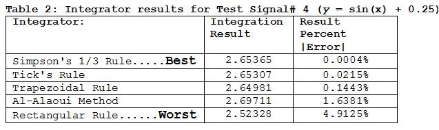
The rightmost column of Table 2 was computed using:

Notice how our measured accuracy ranking of our five digital integrators in the left column of Table 2 is very different than the left column of Table 1. This tells us our initial Table 1 assumptions of integrator accuracy should now be viewed with great suspicion.
The integration accuracy percent absolute error results for Test Signal# 4, the rightmost column of Table 2, are represented by the center column of symbols in Figure 4. Our five digital integrators' accuracy error results for the remaining six Test Signals in Appendix B are also shown in Figure 4.
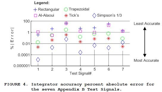
We see in Figure 4 that in general, but not always, the Simpson's 1/3 Rule integration method produced more accurate results than the other four digital integrators. In addition, surprisingly, given its minimal frequency-domain error curve in Figure 3 the Al-Alaoui integration method performed rather poorly.
Conclusion
My empirical testing, whose results are given in Figure 4, shows that: A digital integrator's accuracy performance is not solely a function of its frequency-domain response. It's performance is also profoundly dependent upon the integrator's input signal. Thus our naive integrator performance ranking in Table 1, based solely on the frequency-domain error curves in Figure 3, is not valid.
When I say "dependent upon the integrator's input signal" I mean dependent, in an unpredictable way, on the input signal's:

References
[1] Dyer, S. and Dyer, J., "Numerical Integration", IEEE Instrumentation & Measurement Magazine, April, 2008, pp. 47‑49. Available online: https://www.researchgate.net/publication/3421163_bythenumbers_-_Numerical_integration
[2] Arias-Trujillo, J., Blázquez, R., and López-Querol, S., "Frequency-Domain Assessment of Integration Schemes for Earthquake Engineering Problems", Hindawi Publishing Corporation Mathematical Problems in Engineering, Volume 2015, Article ID 259530. Available online: http://downloads.hindawi.com/journals/mpe/2015/259530.pdf
[3] Al-Alaoui, M., "Novel Digital Integrator and Differentiator", Electronic Letters, Feb. 18, 1993, Vol. 29, No. 4, pp. 376‑379. Available online: https://feaweb.aub.edu.lb/research/dsaf/Publications/12.pdf
Appendix A: Digital Integrators
This appendix describes the five digital integrators whose accuracy performance is investigated in this blog.
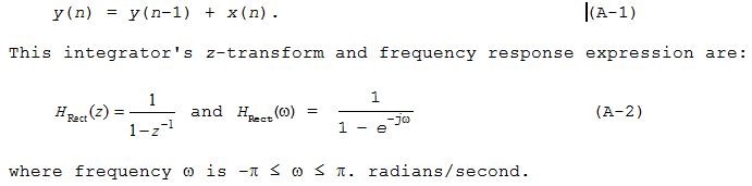
Rectangular Rule Integration
The Rectangular Rule (also called the "Backward Rectangular Rule") integration method is defined by the following difference equation:
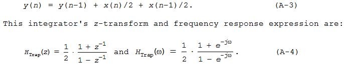
Trapezoidal Rule Integration
The Trapezoidal Rule (also known as the "Tustin Rule") integration method is defined by the following difference equation:
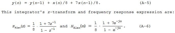
Al-Alaoui Integration
The Al-Alaoui integration method is defined by the following difference equation:
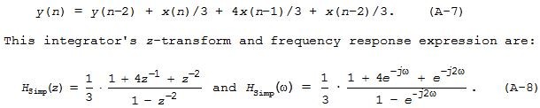
Simpson's 1/3 Rule Integration
The Simpson's 1/3 Rule integration method is defined by the following difference equation:
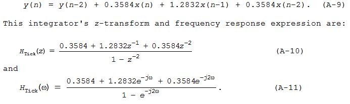
Tick's Rule Integration
The Tick's Rule integration method is defined by the following difference equation:
Appendix B: Test Signals
The seven discrete Test Signals applied to our five digital integrators are shown by the dots in the top y(x) panels of Figure B‑1. Each integrator estimates the definite integral defined by:

where signal y is a function of independent variable x. The a and b limits values for each Test Signal are given in Figure B‑1. For reference, below each 25‑sample discrete y(x) sequence in Figure B‑1 is its positive-frequency |Y($\omega$)| spectral magnitude where frequency variable $\omega$ is measured in radians/sample.
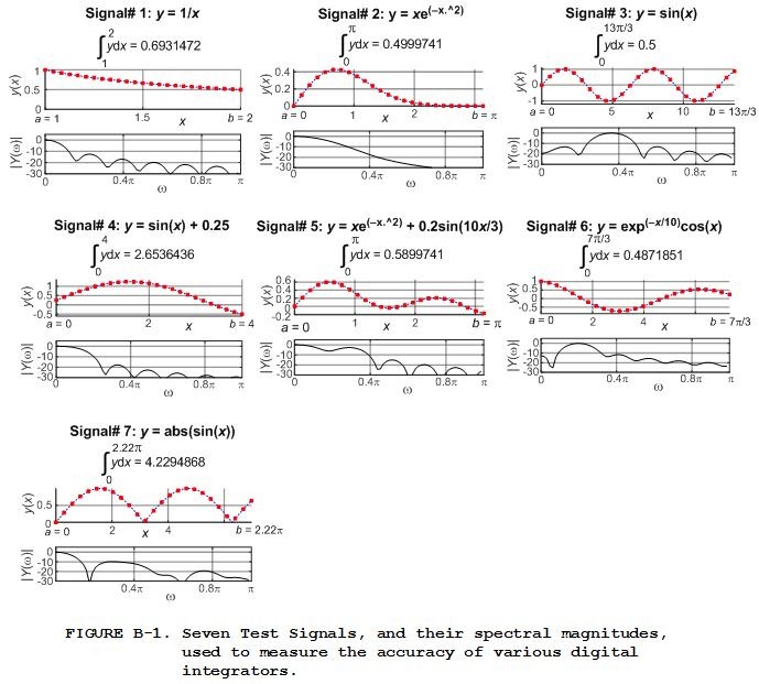
These seven test signals were chosen because their true definite integrals are easily found using integral calculus.
- Comments
- Write a Comment Select to add a comment
Rick:
First comment from a Long-Time Lurker. Thanks for your many excellent postings.
I believe you meant to say from x = 0 to x = 4 radians in 25 steps.
The results certainly depend on the signal shape.
You probably thought it was too obvious to state that the results for any given signal also depend on the ratio of the sample rate to the bandwidth of the signal. For example, your signal 4 using Simpsons with 100 samples results in 2.288e-6 percent error (compared to the integral in DP) for 100 samples over 0:4 radians.
LT1

Hi LT1. Thanks for "catching" that typo of mine!
Your last paragraph is absolutely correct and has caused me to add a few words of text to my 'Conclusion' section. In my integrator accuracy modeling I found that the an innocent-looking change to a test input signal may have a very noticeable, and to me unpredictable, change in the integrator's output value.
LT1, did you know there is a way to predict the maximum error when using the Trapezoidal Rule integrator to integrate a discrete version of a mathematical function. That prediction doesn't give us the error in integrating a math function, but rather gives us a value for which the integration error will never exceed. Unfortunately that error "bound" analysis requires that we first use calculus to find the 2nd derivative of the input math function.
I wonder if that Trapezoidal Rule error bound analysis can, somehow, be used to predict the max error when integrating real-world signals such as the output of an accelerometer.
Rick,
Yes, Et= (-h^3/12)f''(xi), but I much prefer Simpsons for which
Es= (-h^3/90)f''''(xi) with h the panel size and xi an interior point between the limits of integration.
I wonder why one would need the integral of position, but as a non-nav guy, I can't be of any help (sorry), except perhaps to say I always reach for Simpsons because of the behavior implied above. I avoid higher order (4th +) polynomial approximations because of the susceptability to noise and measurement error (oscillations).
LT1
PS, I was logged in and hit submit reply earlier, but it told me that I had to be logged in to reply and sent my reply to the bit bucket in the sky. Frustrating! Then I logged out and logged back in to generate this.
Hi LT1. Just for my own education, what does the phrase "non-nav" mean?
Sorry you had trouble posting a Reply. I've had some of my replies disappear in the past because, in the middle of typing a Reply I clicked on another web page window. Now I'm much more careful when typing a new Reply.
Hi Rick,
Sorry for the abbreviation. I should have simply said that I have no experience with navigation systems.
Thanks for the hint.
LT1

Hi Rick,
Thanks for the blog.
I don't see any comment on dc gain in any of the integrators. For example the rectangular case has dc gain of 45 dB. Wouldn't a practical integrator need control of this gain. This is where loop alpha factor comes into action.
Regards
Kaz
Would the dc gain for the rectangular case not be infinite
yes it is infinite but I quoted 45 dB near dc as a concession
Hi kaz. Yes, you're right. The integrators' z-transforms have a pole at z = 1, right on the unit circle. So their unit impulse responses are non-zero and infinite in length and this gives the integrators a DC gain of infinity. But because these integrators are used to integrate a finite-length sequence of samples, the integrators' single output value will be finite in value.
Hi Rick,
A couple of points.
1) The ideal integrator is the one that does my job.
I don't see there is a specific meaning for ideal.
2) If we take any set of filters targeting same cutoff e.g LP FIR, we end up with different transition curves. As such the output for a given input will be affected by how that input is sliced under the transition curve.
Kaz
Hi kaz.
Please forgive me. I don't understand your Sept. 29, 2019 Comment.
Hi Rick,
I have no experience in numerical integration so sorry for the naive questions.
In your 'benchmark' Simpsons 1/3 is performing best, I was wondering if results would look different if you used a denser sampling of the x-axis. Would you expect the relative rating of the integrators to be dependent on the 'sampling frequency'?
Should one be concerned about stability issues considering the pole at z=1? I previously remember you wrote something on the stability of the Goertzel filter which also has a pole on the unit circle.
Why is it that there is no trapezoidal differentiator or tick's rule differentiator that is just the inverse of the integration rules?
Your questions are not at all naive. They're darned good questions. Questions like yours are how discoveries are made!
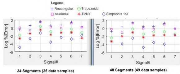
[Question#1] Well, we should expect the accuracy performance of the integrators to improve if we increase the number of data samples (increase the samplng frequency) in our integration estimations. And that turns out to be true.
The left panel below is my blog's Figure 4 accuracy results for 25 data samples. The right panel shows the improved accuracy results for 49 data samples (double the Figure 4 sampling frequency). In the right panel the Log%|Error| for the Simpson integrator for Test Signal# 1 is more negative than -6 so its blue diamond symbol isn't shown in that plot.
[Question# 2] No, there's no worry about stability with these integrators. The integrators' z-transforms have a pole at z = 1, right on the unit circle. So their unit impulse responses are non-zero and infinite in length. But the impulse response sample values do not increase as time passes so the integrators are "marginally stable." But because these integrators are used to integrate a finite-length sequence of samples, the integrators' single output value will be finite in value.
[Question# 3] Now that is a GREAT question. Sadly, I don't have an answer for you. But after I'm finished watching 'WWE Smackdown' on the boob tube I'll try to come up with an answer.
Thanks Rick,
As we can see from your Fig 2 and 3 we should expect larger differences in performance the more high frequency content is in the input. Also it could be interesting to see if all the different rules actually converge to the true value as sampling frequency goes to infinity.
I believe there are applications where such integrators are not used on short input sequences but could run on very long input sequences (such as an audio input stream). And I think that Goertzel filters 'normally' has the pole(s) adjusted off the unit circle by a tiny value for stability reasons. So I was just wondering if the same would apply to the integrators. But for some reason this seems to not be the case.
Looking forward to read your blog on trapezoidal differentiator ;)
Yes, the different integration methods do converge toward a true definite integral value as sampling frequency is increased.
Years ago I thought a Goertzel filter was only marginally stable. But I was wrong. A Goertzel filter is guaranteed-stable as I explained at:
https://www.dsprelated.com/showarticle/796.php
There's no worry about stability with the integrators in my blog as I explained in my above Sept. 30 reply to your Question# 2.
I'm experimenting with your notions of Trapezoidal and Simpson differentiators. But I making no useful progress so far.
Hi Rick,
Not sure if you are looking into this anymore but I just want to mention something regarding stability and then you can correct if something is invalid/incorrect.
The Goertel filter and the trapezoidal integrator are equivalent (same transfer functions) for the case when the Goertzel is configured for the DC bin (pole at 1) and their impulse responses are constant. For the case that the Goertzel is not computing the DC bin its impulse response oscillates forever with no decay. No stability issues as long as we make sure that coefficient quantization does not push the pole outside the unit circle and a bounded input results in a bounded output. However in contrast to the trapezoidal integrator the Goertzel needs multiplication with its coefficient to its state variable (y[n-1]) this is not needed in the trapezoidal integrator. So if the center frequency of the Goertzel is close to DC then numerical stability can be an issue because of round-off errors.
From a DSP point of view I think that both the Trapezoidal integrator and the 'Trapezoidal differentiator' should somehow be treated with some caution when it comes to stability. Because they both have their poles on the unit circle their steady-state responses and transient-responses are merged, the transient (not sure if this is the correct name as it continues forever) doesn't die out. What I mean by this is that if stability of a filter is thought of as 'the filter not generating tones not present in the input' then both the Trapezoidal integrator and the 'Trapezoidal differentiator' can be thought of as not stable. The Trapezoidal integrator generates a DC offset and the 'Trapezoidal differentiator' generates a tone at fs/2 (nyquist). This tone added by the 'Trapezoidal differentiator' is perhaps what leaves it very inattractive as the output looks very noisy.
A pole on the unit circle is a tricky thing.
Regarding your 3rd paragraph, neither the trapezoidal integrator nor the Goertzel filter will ever be unstable. Stability of a filter is *NOT* thought of as 'the filter not generating tones not present in the input'. The concept of network "linearity" is associated with a filter not generating tones not present in the input.
Hi Rick. Sorry, yes you are correct. It's the rectangular integrator and the Goertzel (as specified in eq [5] here on wiki https://en.wikipedia.org/wiki/Goertzel_algorithm) that are equivalent at DC. Just wanted to mention that there is a possibility of numerical stability but I don't think there is any point in discussing this. And you are of course correct that I should not have used the term unstable in the 2nd paragraph.
Hi niarn. Thanks for the wiki Goertzel web link. I don't recall ever visiting that interesting web page before.

Rick,
I thought a perfect digital integrator was trivial: H(z) = 1 / (1 - z^(-1)). It appears you are trying to make a digital filter that mimics the frequency response of a perfect analog filter from 0 to Fs/2. That could be useful for some purposes, but is it "ideal?"
--Randy
Hi Randy. (Hope you're doin' well.)
Your H(z) equation is identical to my Eq. (A-2).
The point of my blog is to contradict the traditional belief that the "best" digital integrator is the one whose freq magnitude response most closely matches an ideal integrator's 1/(j times omega) freq magnitude response (my blog's Eq. (1)).
The proof that such a belief is not valid is the performance of the Al-Alaoui Method integrator. The Al-Alaoui integrator's freq magnitude response most closely matches an ideal integrator's freq magnitude response, as shown by my blog's Figure 2, but the Al-Alaoui integrator's accuracy performance is among the worst of all the integrators.
Hi Rick,
that's a pretty cool analysis. I would just like to ask if you could plot Figure 3 while taking the absolute value of the imaginary part of the functions? And try to zoom around ω=0. The final value of y[n] should be jω*Y(ω) evaluated at ω=0, so it'd make sense to see which of these is most accurate at those points.
Hi NariOX.
I'm a bit confused. Can you give me more explanation of what you mean by
"The final value of y[n] should be jω*Y(ω)"?
Sorry Rick, I got my equations from CT and DT mixed up. In any case, I was referring to the final value theorem: https://en.wikipedia.org/wiki/Final_value_theorem. The right equation should be (1-z)(H(z)).
Since we are just looking at the final value of the integrals, the frequency response does not matter as much as the accuracy around ω=0 (z->1)
I've made a few plots to show this. The first is comparing rectangular approximation to trapezoid:
https://www.wolframalpha.com/input/?i=plot+%28z-1%...
Notice how the trapezoid function is much smoother/smaller around z=1.
Now, if add Al-Alaoui:
https://www.wolframalpha.com/input/?i=plot+%28z-1%...
Notice that it is about the same amount off as rectangular (which explains why their performance is about the same in your tests).
Finally, look at trapezoid compared to Simpson's:
Simpson's is significantly smoother. I haven't done the same for Tick's, but I haven't had the time.
What intrigues me is that for function 2, I'd expect the trapezoid and rectangular to give the same result (as the first sample is 0 and the last samples is close to 0). I wonder if numerical precision is also playing a role in your results. Maybe we could try with signals whose values can be expressed as a sum of negative powers of 2 (maybe x*2^(-x) or x*2^(-x^2), etc). Your function 1 follows this pattern, which might explain why the results are the best (for all methods but Al-Alaoui).
Sorry for the long reply. I hope this makes sense.
It appears that your 2nd and 4th https links are the same.
Does the curve you generated for the rectangular rule integrator imply that the y(n) output sample, for very large values of n, is equal to zero?
Dumb Question: Why is there a logarithm in the equation for the rectangular rule integrator's z-transform equation?
Hi Rick,
sorry, you are right. I've edited the 4th link.
And also, sorry, I should have explained the plots a little better. Not a dumb question at all! I did something similar to your Eq. 2, where I normalized the equations to the 1/jω. Now, to convert that to z-domain, I used 1/log(z), (as (1/log(exp(jω) = 1/jω).
So, the idea is that the mean of the relative errors should be 0 (meaning all of these are unbiased estimators). But I haven't tried to analyze the variance (which would probably be more insightful in this matter). My guess is that the variance depends on the number of samples taken, but I won't have time to dig deeper for another few weeks.
Hope this makes sense
Hi NariOX. Thank you for bringing up the topic of the Final Value Theorem here. It's a topic, that I don't recall thinking about before, where the region of convergence (ROC) of a discrete sequence must be considered. I'm still studying this topic but at first glance it appears that the Final Value Theorem is not applicable for the Simpson or Tick's Rule integrators. My study continues. Thanks again.
Hmm. That's intriguing, I had not looked at Simpson's rule's FVM. Tick's does work.
Part of the issue (I believe) is that none of these signals are bandlimited, so some of the assumptions we are making don't apply to the signals. But I'm far from understanding how all of these pieces connect together.
If I recall correctly, Simpson's rule
comes from treating the samples as samples of a polynomial (using
Lagrangian polynomials). But I had never looked at them from the
perspective of signals (I always just used the rectangular rule), so
this is all uncharted territory for me.
The Rectangular rule is equivalent of applying the integral to Zero-Order-Hold, or, in other terms, a zero order polynomial. The trapezoid is equivalent to linear interpolation, so errors arise if the interpolated function is of order higher than 2. The "ideal" integrator would be equivalent of doing sinc interpolation (which would be "perfect" if the signals are bandlimited).
Maybe a better way to look at these would be to plot the output of the integrating filters and see how they compare to the true integral.
Hi NariOX. It's the Final Value Theorem (FVT) that intrigues me now. As I understand the FVT, I was able to obtain sensible FVT results for the Rectangular Rule, Trapezoidal Rule, and Al-Alaoui Method integrators.
However, I was NOT able to obtain sensible FVT results for the Simpson's 1/3 Rule or Tick's Rule integrators. And I think that's because the region of convergence of the product of (z-1) times the Simpson and Tick's integrators' z-transforms do not include the z-plane unit circle.
NariOX, using the FVT, what numerical value did you obtain for the "final value" for a Tick's Rule integrator? I computed a final value of one (unity), which I believe is not correct.Hi Rick,
this has been really fun. I figured why the Simpson's rule was not converging to 1. Equation A-8 has an error. The denominator on the equation on the right hand side should be 1/3 (like the equation in the center), but it has 1/8.
The FVT for just the H(z)'s should be 1, because that would be the integral of the Kronecker delta (impulse function). In continuous time, that'd be equivalent of the integral of the sinc function, which is also 1 (or of Dirac's delta, in the non-bandlimited case)
Hi NariOX. Thanks a lot for catching that "typo" in my blog. (I've corrected it.)
Yes, this thread of ours has been fun. And it's forced me to reexamine the accuracy of the Simpsnon's 1/3 Rule integrator, which has been educational for me.
For the Simpson's 1/3 Rule integrator, using the FVT yields a value of one. But the impulse response of the integrator is not asymptotic-- it's a never-ending oscillating sequence (oscillating between two positive values).
I believe the reason we can't obtain sensible FVT results for the Simpson's 1/3 Rule integrator is because the region of convergence of the product of (z-1) times the Simpson integrators' z-transform does not include the z-plane unit circle.
Dear Sir
please check your results for the AI-Alaoui intergrator because the A-5 and A-6 equations are not correct.
According to the original article of AI-Alaoui [3], the transfer function of the integrator, see the equation (4) of the article, is:
H(z) =T* 7/8 * (z + 1/7) / (z-1)
that brings to the final equation :
y(n) = y(n-1) + T*[ 7/8*x(n) + 1/8 * x(n-1) ]
so the weights for x(n) and x(n-1) are swapped bringing more weight
for x(n) respect to x(n-1)
best regards
Dear rocky75.
Al-Alaoui discussed two integrators. He discussed what he called his "New nonminimum phase digital integrator" described by his Equation (3). Then he discussed what he called his "New minimum phase digital integrator" described by his Equation (4).
I modeled both of Al-Alaoui's integrators and found no meaningful difference between their performances. So I only discussed his "New nonminimum phase digital integrator" in my blog here.
To post reply to a comment, click on the 'reply' button attached to each comment. To post a new comment (not a reply to a comment) check out the 'Write a Comment' tab at the top of the comments.
Please login (on the right) if you already have an account on this platform.
Otherwise, please use this form to register (free) an join one of the largest online community for Electrical/Embedded/DSP/FPGA/ML engineers:


