Third-Order Distortion of a Digitally-Modulated Signal

• Matlab
• Tutorials

In the following analysis, we assume that signal phase at the amplifier output is not a function of amplitude.  With this assumption, the output y of a non-ideal amplifier can be written as a power series of the input signal x:

$$y= k_1x+k_2x^2+k_3x^3+k_4x^4+k_5x^5+ \cdots \qquad (1) $$

The coefficients k_i are real.  Right off the bat, we’ll simply ignore all the even-order terms.  There are two reasons why we can usually get away with this:

• The frequency components of even-order distortion typically do not fall near the desired signal and can thus be removed by filtering (See Appendix A of the PDF version).  This does not hold for wideband signals, though.
• For moderate signal levels, the amplifier output is usually nearly half-wave symmetrical [1,2], which causes the even-order frequency components to be small.

Once again assuming moderate signal level, we expect the 3^rd order term to dominate over the higher-order terms.  If we eliminate those terms, we’re left with the following equation, where, for simplicity, we have set k₁= 1:

$$y= x+k_3x^3 \qquad (2) $$

Note that the output signal y of this model has the same phase as the input signal x.  As an example of such a distortion characteristic, Figure 1a plots y vs x for $y=x-.03x^3.$  Clearly, this does not represent the characteristic of a real amplifier, whose output amplitude would reach a clipping limit rather than changing sign and increasing drastically for larger |x|.  We would need the higher-order terms in Equation 1 to produce a realistic characteristic.  Nevertheless, this is a useful example if we keep |x| less than 3 or so.

In Equation 2, the linear gain of the amplifier is 1.0.  When the coefficient k₃ is negative, the total gain is reduced below 1.0 as |x| increases, as can be seen from the slope in Figure 1a.  This phenomenon is called gain compression.  For our example, Figure 1b shows the effect of gain compression on a sinewave with peak amplitude of 2.5 volts.

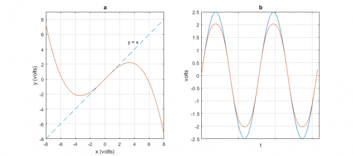
Figure 1.  a. The function y = x - .03x³.     b. Sinewave input x and distorted output y (orange)

Why third-order distortion matters

To see the effect of third-order distortion in the frequency domain, we apply two tones at different frequencies to the nonlinearity.  In the following Matlab code, x is the sum of two sinusoids with frequencies f₁ and f₂.  The power spectral density (PSD) of y in dBm/bin is computed using the function psd_simple2.m (See Appendix B in the PDF version).  The PSD calculation assumes a load resistance of 50 ohms.

    fs= 100;                % Hz sample frequency
    Ts= 1/fs;
    f1= 10; f2= 12;         % Hz frequencies of tones
    A= 0.707;               % V amplitude of tones
    N= 2048;                % number of samples
    n= 0:N-1;
    x= A*sin(2*pi*f1*n*Ts) + A*sin(2*pi*f2*n*Ts);    % input signal
    y= x -.03*x.^3;                                % nonlinearity
    [PdBm,f]= psd_simple2(y,N,fs);                 % dBm/bin power spectral density
    plot(f,PdBm),grid, axis([0 fs/2 -70 10])

The spectrum of y is plotted in Figure 2.  As shown, the 3^rd- order nonlinearity creates distortion components at 2f₁ – f₂ and 2f₂ – f₁, as well as harmonic components at and near the 3^rd harmonics of f₁ and f₂ [3].  We refer to the components near f₁ and f₂ as Third-Order Intermodulation Distortion (Third-Order IMD or IMD3).  If a signal has closely spaced frequency components, the intermodulation components fall close to the signal itself, and cannot normally be removed by filtering.  Like noise, third-order distortion is just something we have to live with.  For the most part, system designers deal with third-order distortion by using amplifiers with adequate linearity.  Amplifier data sheets often include specifications for two-tone third-order IMD. Note that for a given amplifier, you can estimate k₃ by adjusting its value in the Matlab code until the simulated two-tone IMD3 approximates the measured value.

The amplitude of the intermodulation components varies as x³.  Since log₁₀(x³) = 3log₁₀x, their dB value changes 3 dB for every 1 dB change in the signal level.  For example, in Figure 3, reducing the level of the tones by 10 dB causes the intermodulation components to drop by 30 dB.  This is a net drop of 20 dB with respect to the level of the tones.

We have assumed the above discrete-time model adequately represents distortion in continuous-time components, such as amplifiers.  To be valid, the model must have sample frequency sufficiently high to prevent aliasing of the 3^rd harmonics.  In our example, the highest component was 3*f₂ = 36 Hz, which is below the Nyquist frequency of 50 Hz.  The model is not a computationally efficient way to estimate distortion.  A more efficient approach uses a complex-baseband model.  As already mentioned, we also assumed that signal phase at the amplifier output is not a function of amplitude (no AM-to-PM conversion).  For discussions of complex baseband and AM-to-PM models, see [4,5].

Finally, note that the amplitude of each tone in the above Matlab code is 6.7 dBm at the output of the nonlinearity.  However, the amplitude displayed in Figure 2 is only about 4.3 dBm, due to the processing loss of the Kaiser window used in psd_simple2.m.

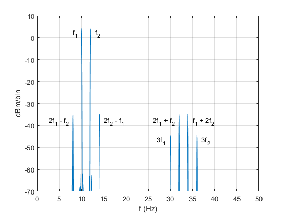
Figure 2.  Two-tone third-order intermodulation distortion and third harmonic distortion.

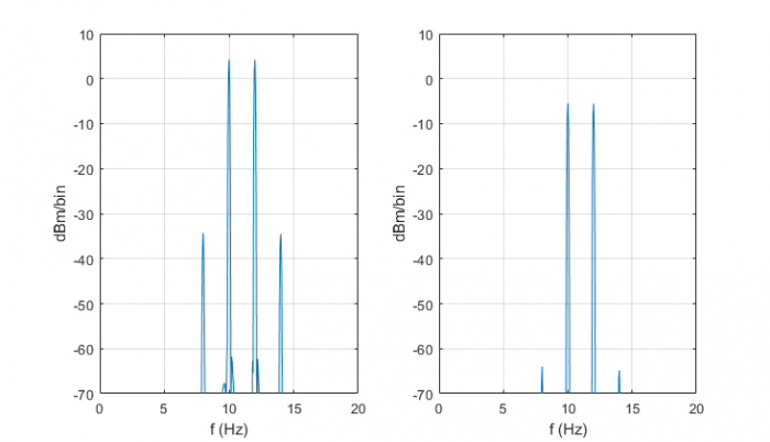
Figure 3.  Change in intermodulation components is 30 dB for 10 dB change in tone level.  (20 dB change relative to the level of the tones).

Third-order distortion of a QAM signal

Here we’ll simulate distortion of a QAM signal, but our model could be used for other modulation types as well.  In order to use Equation 2 to model distortion of QAM, we need to generate a real QAM signal centered at a carrier frequency f₀.  Appendix C in the PDF version lists a Matlab function qam_tx_real.m that we’ll use to generate the QAM signal.  For our example, we’ll apply the signal to an amplifier with 10 dB of gain:  20log₁₀G = 10.  Solving for voltage gain G, we get $G=\sqrt{10}.$  Modifying Equation 2 to replace x with Gx, we have:

$$y=Gx+k_3(Gx)^3 \qquad(3)$$

The following Matlab code applies a QAM-16 signal (with Gaussian noise added) to Equation 3, and computes the spectrum of the input QAM signal and output QAM signal.  Coefficient k₃ is -.03.The input signal level is approximately 0 dBm and the output signal level is approximately 10 dBm (10 mW).

    fs= 100;                          % Hz sample frequency
    f0= 12;                           % Hz carrier frequency
    M= 16;                            % QAM order
    R= 50;                            % ohms load resistance
    A= 0.415;                         % amplitude scale factor
    N= 2048;                          % number of QAM symbols
    x= A*qam_tx_real(M,N,f0,fs);      % QAM modulator
    x= x + .001*randn(1,16*N);        % add gaussian noise to signal
    G= sqrt(10);                      % voltage gain of amplifier
    y= G*x - .03*(G*x).^3;            % amplifier characteristic
    u= y(200:end);
    L= length(u);
    Pav= 1000*(sum(u.^2)/R)/L            % mW output power of amplifier
    PdBm= 10*log10(Pav)                  % dBm output power of amplifier
    [PdBm_in,f]= psd_simple2(x,N,fs);    % dBm/binpower spectral density
    [PdBm_out,f]= psd_simple2(y,N,fs);
    plot(f,PdBm_in,f,PdBm_out),grid, axis([0 fs/2 -80 0])

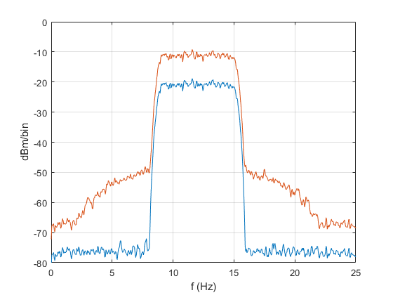
The input and output spectra of the QAM signal are shown in Figure 4.  The third-order distortion has caused spreading, or “regrowth” of the output spectrum, as well as a haystack of distortion centered at 3f₀.    Again, we used a sample rate high enough to place the components around 3f₀ safely below the Nyquist frequency.

The output spectrum with regrowth occupies a bandwidth of about 20 Hz, which is roughly three times the signal bandwidth.  (Compare this to the frequency spacing of the discrete distortion components in Figure 2, which is exactly three times the frequency spacing of the input tones).  Note, however, that as the amplifier is driven harder, the higher-order distortion components become significant.  This causes the spectrum spread to increase beyond what our third-order model predicts.

The spectral regrowth can cause interference to signals in adjacent channels, so system specifications often include requirements for Adjacent Channel Power Ratio (ACPR) [6].  You can compute adjacent channel power from the simulation by summing the PSD’s power per bin over the adjacent channel’s bandwidth.

Besides causing spectral regrowth, third-order IMD distorts the constellation of the received QAM symbols.  Figure 5 shows the spectrum and receiver constellation for a 13 dBm (20 mW) QAM-16 signal with the same value of k₃ as the previous case.  The spectral regrowth level with respect to the signal level is about 6 dB higher, and the constellation is distorted due to gain compression, which has the greatest effect on the corner points.  The constellation’s Modulation Error Ratio [7] is about 30.5 dB, compared to 50.5 dB for the case with no distortion.

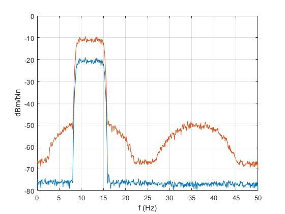
Figure 4.  Modeled QAM-16 spectra at input and output of amplifier with 3^rd-order distortion.

Blue:  input signal (0 dBm).    Orange:  output signal (10 dBm).

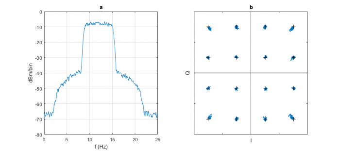
Figure 5.  Modeled QAM-16 amplifier output spectrum (a) and receiver constellation (b).

Amplifier output signal power = 13 dBm.

For Appendices, see the PDF version.

References

1.  Hayt, William H., et al, Engineering Circuit Analysis, Eighth Ed., McGraw-Hill, 2012, p 745 – 747.

2.  Krambeck, Donald, “The Effect of Symmetry on the Fourier Coefficients”, allaboutcircuits.com, February, 2016,

https://www.allaboutcircuits.com/technical-articles/the-effect-of-symmetry-on-the-fourier-coefficients/

3.  Henn, Christian, “Intermodulation Distortion (IMD)”, Burr-Brown (now Texas Instruments), 1994,

http://www.ti.com/lit/an/sboa077/sboa077.pdf

4.  Tranter, William H., et. al., Principles of Communication Systems Simulation, Prentice Hall, 2004, Ch. 12.

5.  Nentwig, Markus, “Understanding Radio Frequency Distortion, DSPRelated.com, September, 2010,

https://www.dsprelated.com/showarticle/108.php

6.  “Optimizing IP3 and ACPR Measurements”, National Instruments,

http://www.ni.com/pdf/en/Optimizing_IP3_and_ACPR_Measurements_With_the_PXIe_5668R.pdf

7.  Robertson, Neil, “Compute Modulation Error Ratio (MER) for QAM”, DSPRelated.com, November, 2019, https://www.dsprelated.com/blogs-1/nf/Neil_Robertson.php

8.  Robertson, Neil, “A Simplified Matlab Function for Power Spectral Density”, DSPRelated.com, March, 2020, https://www.dsprelated.com/showarticle/1333.php

9.  Robertson, Neil, “Evaluate Window Functions for the Discrete Fourier Transform”, DSPRelated.com, December, 2018, https://www.dsprelated.com/showarticle/1211.php

Neil Robertson           June, 2020

Sign in