Digital PLL's -- Part 1

• Matlab
• Tutorials

1. Introduction

Figure 1.1 is a block diagram of a digital PLL (DPLL).  The purpose of the DPLL is to lock the phase of a numerically controlled oscillator (NCO) to a reference signal.  The loop includes a phase detector to compute phase error and a loop filter to set loop dynamic performance.  The output of the loop filter controls the frequency and phase of the NCO, driving the phase error to zero.

One application of the DPLL is to recover the timing in a digital demodulator.  In this case, the phase detector computes the phase error from the complex I/Q signal.  Another application would be to lock to an external sine wave that is captured by an A/D converter.

A basic DPLL model is shown in Figure 1.2.  In this model, the reference signal and the NCO output are both phases.  The phase error is simply the difference of the reference phase and the NCO phase.  This is the DPLL model we will use here.  (As an example of a reference phase, if a reference sine wave were applied to a Hilbert transformer, the phase of the Hilbert I/Q output could be used to generate the reference phase: phi_ref= arctan(Q/I) ).  

We will use Matlab to model the DPLL in the time and frequency domains (Simulink is also a good tool for modeling a DPLL in the time domain).  Part 1 discusses the time domain model; the frequency domain model will be covered in Part 2.  The frequency domain model will allow us to calculate the loop filter parameters to give the desired bandwidth and damping, but it is a linear model and cannot predict acquisition behavior.  The time domain model can be made almost identical to the gate-level system, and as such, is able to model acquisition.  I discuss a PLL model whose reference input is a sinusoid (rather than a phase) in Part 3.

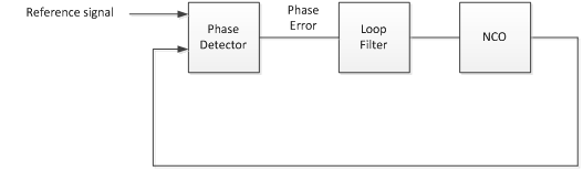
Figure 1.1  Digital PLL

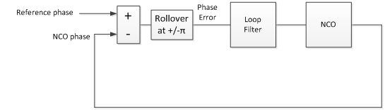
Figure 1.2  Digital PLL model using phase signals

2. Components of the DPLL Time domain model

As shown in Figure 1.2, the DPLL contains an NCO, phase detector, and a loop filter.  We now describe these blocks for a 2^nd order PLL [1, 2].  To keep things simple, all blocks use the same sample frequency.  This discussion deals with the phase of sampled sine waves.  For background, see Appendix B.

The NCO

The phase of a sine wave is given by:

phi= 2*pi*mod(f*n*Ts,1)

Here f is the frequency, n is sample index, and T_s is sample time.  To create an NCO, we just implement the above equation.  But rather than generate phase in radians, we remove the 2*pi to give phase in cycles.  Then the range of phase (renamed u) is 0 to 1.

u = mod(f*n*Ts,1);      % cycles

The implementation in Figure 2.1 is an accumulator that rolls over when x >1, with input f*T_s = f/f_s.  The output u is phase in cycles.  The output y is a sine wave at frequency = f.  The cosine function is generated using a lookup table or CORDIC algorithm. 

For our DPLL we make two modifications, as shown in Figure 2.2.  We add input Vtune and scaling K_nco to allow an offset from the center frequency, f.  Typically, K_nco << 1.  Also, we removed the sinusoidal output; only the phase output is needed in the model.  With the sine output removed, we refer to the NCO as a phase accumulator.

The difference equations for the phase accumulator are simply:

x = f*Ts + u(n-1) + vtune(n-1)*Knco;     % cycles NCO phase
u(n) = mod(x,1);                         % cycles NCO phase mod 1

A note on quantization:  In a digital implementation, u must be quantized to a reasonable number of bits.  For simplicity, we have not included quantization in this and subsequent models, but it can easily be added.

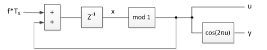
Figure 2.1.  Basic NCO

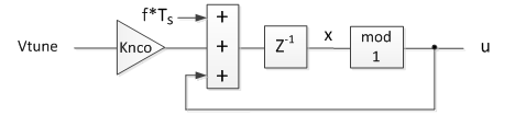
Figure 2.2.  Phase Accumulator for DPLL.   u = phase in cycles.

The Phase Detector

The phase detector is shown in figure 2.3.  It performs a difference, then a rollover function when the phase crosses +/- ½ cycle (+/- π radians).  The difference equations are:

pe= ref_phase(n-1) - u(n-1);     % phase error
pe= 2*(mod(pe+1/2,1) - 1/2);     % wrap if phase crosses +/- 1/2 cycle
phase_error(n) = pe;

The output of the phase detector has a range of +/-1 for an input phase difference of 1 cycle.  Thus the phase detector gain is:

K_p = 2     in units of cycle^-1.

A plot of phase detector output vs. phase error is shown in Figure 2.4.

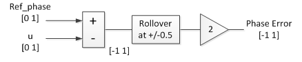
Figure 2.3  Phase Detector

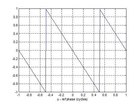
Figure 2.4  Phase Detector Characteristic

The Loop Filter

For a 2^nd order loop, the loop filter consists of a proportional gain K_L summed with an integrator having gain K_I.  It is called a Proportional + Integral or Lead-Lag filter.  The difference equations are:

int(n) = KI*pe + int(n-1);     % integrator
vtune(n) = int(n) + KL*pe;     % loop filter output

where pe is the phase error.  KL and KI determine the damping and natural frequency of the PLL.  We will show how to calculate KL and KI in Part 2.

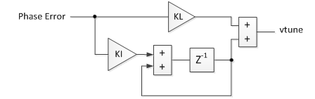
Figure 2.5  Loop Filter

Putting all the components together, the DPLL time domain model is shown in Figure 2.6. 

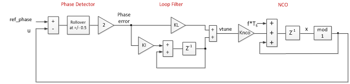
Figure 2.6  DPLL Time Domain Model Block Diagram

3. Example Cases of DPLL Time Domain model

The Matlab script for the time domain DPLL is listed in Appendix A.  The input parameters for the examples are:

f_s                                                    25 MHz
Reference frequency                     8 MHz
Initial reference phase                   0.7 cycles
NCO initial frequency error           -100 ppm or -500 ppm (-800 or -4000 Hz)
K_nco                                                1/4096
N                                                    30,000 or 100,000 samples
f_n                                                    5 kHz or 400 Hz   loop natural frequency.  f_n = ω_n/(2π)
ζ (zeta)                                           1.0                            loop damping coefficient
K_L, K_I                                               calculate from f_n and ζ

The first example has initial frequency error less than loop natural frequency, and the second example has initial frequency error much greater than loop natural frequency.  The formulas for K_L and K_I to obtain the desired natural frequency and damping will be covered in Part 2.

Example 1.  Initial frequency error < Loop natural frequency.  Loop natural frequency = 5 kHz and NCO initial frequency error = -800 Hz.

For this case, the loop behaves as a linear system.  Note we have allowed Vtune to exceed [-1 1], rather than clipping at that level.

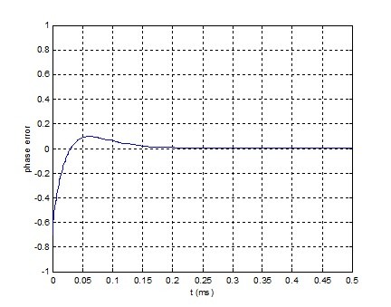
Figure 3.1    Phase error. 

NCO Initial freq error = -800 Hz.  Initial ref phase = 0.7 cycles.  fn = 5 kHz, ζ = 1.0.

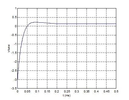
Figure 3.2    Vtune. 

NCO Initial freq error = -800 Hz.  Initial ref phase = 0.7 cycles.  f_n = 5 kHz, ζ = 1.0.

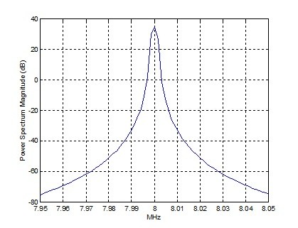
Figure 3.3    Output Spectrum (bin spacing = 25E6/2^14 = 1.53 kHz)

 Example 2.  Initial frequency error >> Loop natural frequency.  Loop natural frequency = 400 Hz and NCO initial frequency error = -4 kHz. 

For this case, the phase detector repeatedly wraps due to the large initial frequency error.  Thus the loop is highly non-linear during acquisition.  Note the time scales of the plots are longer than for the previous example.

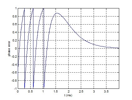
Figure 3.4    Phase error

NCO Initial freq error = -4 kHz.  Initial ref phase = 0.7 cycles.  f_n = 400 Hz, ζ = 1.0.

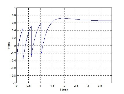
Figure 3.5    Vtune

NCO Initial freq error = -4 kHz.  Initial ref phase = 0.7 cycles.  f_n = 400 Hz, ζ = 1.0.

Appendix A.  Time domain model of DPLL with fn = 5 kHz

% pll_time2.m 6/3/16 nr
% Digital PLL model in time using difference equations.
% fn = 5 kHz NCO initital freq error = -100ppm*8 MHz = -800 Hz
N= 30000;                   % number of samples
fref = 8e6;                 % Hz freq of ref signal
fs= 25e6;                   % Hz sample rate
Ts = 1/fs;                  % s sample time
n= 0:N-1;                   % time index
t= n*Ts*1000                % ms
init_phase = 0.7;           % cycles initial phase of reference signal
ref_phase = fref*n*Ts + init_phase;     % cycles phase of reference signal
ref_phase = mod(ref_phase,1);           % cycles phase mod 1
Knco= 1/4096;                           % NCO gain constant
KI= .0032;                              % loop filter integrator gain
KL= 5.1;                         % loop filter linear (proportional) gain
fnco = fref*(1-100e-6);          % Hz NCO initial frequency
u(1) = 0;
int(1)= 0;
phase_error(1) = -init_phase;
vtune(1) = -init_phase*KL;
% compute difference equations
for n= 2:N;
  % NCO
  x = fnco*Ts + u(n-1) + vtune(n-1)*Knco;     % cycles NCO phase
  u(n) = mod(x,1);                            % cycles NCO phase mod 1
  s = sin(2*pi*u(n-1));                       % NCO sine output
  y(n)= round(2^15*s)/2^15;                   % quantized sine output
  % Phase Detector
  pe= ref_phase(n-1) - u(n-1);                % phase error
  pe= 2*(mod(pe+1/2,1) - 1/2);             % wrap if phase crosses +/- 1/2 cycle
  phase_error(n) = pe;
  % Loop Filter
  int(n) = KI*pe + int(n-1);                 % integrator
  vtune(n) = int(n) + KL*pe;                 % loop filter output
end
plot(t,phase_error),grid
axis([0 0.5 -1 1])
xlabel('t (ms)'),ylabel('phase error'),figure
plot(t,vtune),grid
axis([0 0.5 -3.5 1])
xlabel('t (ms)'),ylabel('vtune'),figure
psd(y(11000:end),2^14,fs/1e6)
axis([7.95 8.05 -80 40]),xlabel('MHz')

Appendix B.    Phase of a sampled sine wave

For a continuous sine wave y = cos(2πft), the phase is 2πft radians.  For a sampled sine wave, we make the following definitions:

N= 50;         % number of samples
fs= 25e6;      % Hz sample frequency
Ts= 1/fs;      % s sample time
f= 1e6;        % Hz sinewave frequency

Noting that 2πf*t  = 2πf*nTs,  the phase is:

n= 0:N-1;             % sample index
phi= 2*pi*f*n*Ts;     % radians phase

To make the phase wrap at phi = 2π, we modify this expression using the modulus function:

phi= 2*pi*mod(f*n*Ts,1);

The phase and its cosine are plotted here:

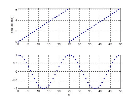
Top:  phase phi of sampled cosine wave (radians).

Bottom:  cos(phi)

References

1.  Gardner, Floyd M., Phaselock Techniques, 3^rd Ed., Wiley-Interscience, 2005, Chapter 4.

2.  Rice, Michael, Digital Communications, a Discrete-Time Approach, Pearson Prentice Hall, 2009, Appendix C.

6/3/2016    Neil Robertson

Sign in