


Find Aliased ADC or DAC Harmonics (with animation)
When a sinewave is applied to a data converter (ADC or DAC), device nonlinearities produce harmonics. If a harmonic frequency is greater than the Nyquist frequency, the harmonic appears as an alias. In this case, it is not at once obvious if a given spur is a harmonic, and if so, its order. In this article, we’ll present Matlab code to simulate the data converter nonlinearities and find the harmonic alias frequencies. Note that Analog Devices has an online tool for the same purpose which does not use simulation [1].
In the lab, many frequency-domain impairments can be measured using the test set-ups shown in Figure 1. For an ADC, we feed a sine to the ADC as shown in Figure 1a, capture the ADC output in memory, and use the captured signal to compute the spectrum using the Discrete Fourier Transform (DFT). For a DAC, we can generate a sine using a numerically-controlled oscillator (NCO) and apply it to the DAC, as shown in Figure 1b. The output is fed to a spectrum analyzer.
Here, our goal is to simulate particular impairments -- harmonics -- and find their frequencies. We can do this by using the model in Figure 2. We generate a sine using an NCO, apply a nonlinearity, then perform the DFT. The resulting spectrum will show the harmonics, including aliased ones, over 0 to fs/2. The model works for either ADC’s or DAC’s.
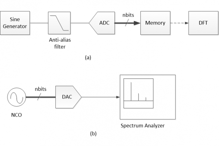
Figure 1. Data converter frequency-domain measurements. a.) ADC b.) DAC
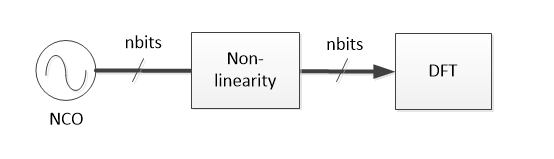
Figure 2. Model for generating and displaying data converter harmonics.
Given NCO output x, the equation for the non-linearity is as follows:
$$ y= x +cx^p \qquad (1) $$
Where c is a constant with absolute value typically much less than one, and p is an integer greater than one. Since our goal is to find just the frequencies, and not the amplitudes, of the harmonics, the exact value of c is arbitrary. Normally, c is negative, which results in gain compression.
The appendix of the PDF version of this article lists the Matlab function adc_dac_harm.m that implements Equation 1. It plots the spectrum of a data converter’s output, given sine frequency f0, sample frequency fs, number of bits, exponent p, and nonlinear coefficient c. The spectrum is plotted over a frequency range of 0 to fs/2. Note that, in the case of a DAC, the function does not model the sinx/x frequency response.
Example without Aliasing
Here is an example using p = 5 without aliasing: i.e., the harmonic falls below fs/2. The nonlinear coefficient is not specified in the function call; it defaults to c = -.05. Matlab code is as follows:
    f0= 1;             % Hz sine frequency
    fs= 20;            % Hz sample frequency
    nbits= 12;         % effective number of bits
    p= 5;              % exponent
    adc_dac_harm(f0,fs,nbits,p);
The spectrum is shown in Figure 3, where we note that there is a 3rd harmonic as well as the 5th harmonic present in the spectrum. This follows from the trigonometric identity:
$$ (sin \theta)^5= \frac58 sin \theta - \frac{5}{16} sin3\theta + \frac{1}{16} sin5\theta \qquad (2) $$
The amplitudes of the harmonics with respect to the fundamental are arbitrary, so the vertical scale is left blank. Note that the 3rd harmonic is larger than the 5th harmonic. In general, Equation 1 results in harmonic amplitude decreasing with harmonic order, so when the harmonics are aliased, you can use this fact to identify the order of each harmonic component.
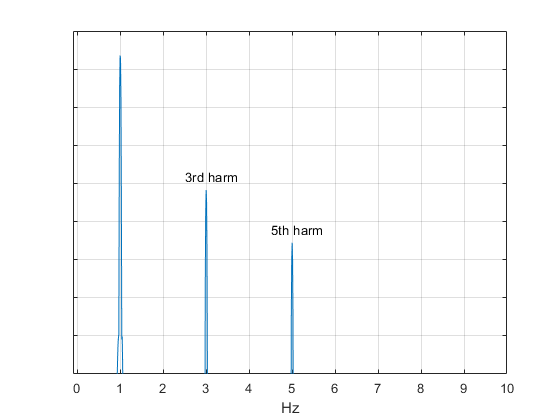
Figure 3. Spectrum with no aliasing. f0 = 1 Hz, fs = 20 Hz, and p = 5.
Examples with Aliasing
Now let’s look at some cases with aliasing. Let f0 = 7 Hz, fs = 20 Hz, and let p = 5. Once again using adc_dac_harm.m, we get the spectrum of Figure 4 (top), which shows the (smaller) 5th harmonic aliasing to 5 Hz and the (larger) 3rd harmonic aliasing to 1 Hz. To check the third harmonic, we note that the aliased harmonic frequency is given by the following equation with p = 3 and k = 1:
$$ f= |pf_0 - kf_s| \qquad (3) $$
$$ f= |3*7 - 20| = 1 Hz$$
Similarly, for the 5th harmonic, with p = 5 and k
= 2, we get:
$$ f= |5*7 - 40| = 5 Hz$$
The bottom plot of Figure 4 uses the same sine and sampling frequencies, with p = 4. The exponent of 4 generates both a 4th and 2nd harmonic, as shown. A dc term is also visible. The two plots of Figure 4 provide all of the harmonics from 2 through 5. You can compare these results to Figure 8 in [2].
Although not needed to display the harmonic frequencies, adc_dac_harm.m includes the quantization inherent in data conversion. To show the quantization noise, let nbits = 9. We want to prevent the noise energy from concentrating on discrete frequencies, so we’ll use a non-integer value of f0: f0 = 7.011 Hz. Keeping p = 5 and fs = 20, and using c = -.01, the spectrum with quantization noise visible is shown in Figure 5.
Finally, if you have ever tested a DAC using the set-up of Figure 1b, you may have seen how the harmonics move across the spectrum (in both directions) as you change the NCO frequency. The mfile movie.m listed in the appendix gives an animated demonstration of this effect for a DAC or ADC (again, DAC sinx/x response is not modeled). The mfile uses fs= 100 Hz, nbits = 9, p = 5, and c = -.01. Run time is roughly 25 seconds.
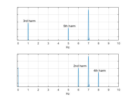
Figure 4. Spectra for f0 = 7 Hz and fs = 20 Hz. Top: p = 5. Bottom: p = 4.
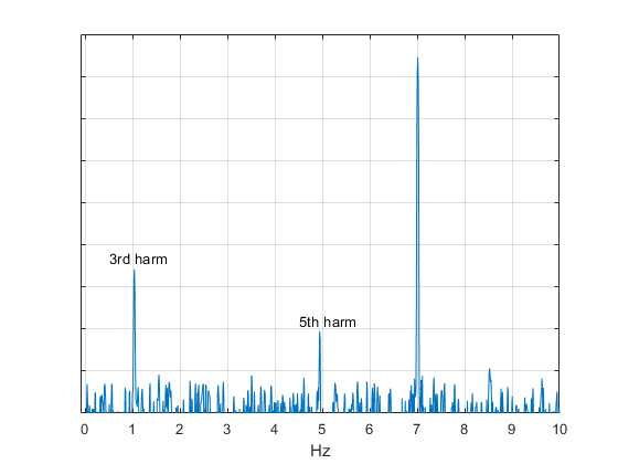
Figure 5. Spectrum with quantization noise visible.
f0 = 7.011 Hz, fs = 20 Hz, p = 5, and c= -.01, with nbits = 9.
For the appendix, see the PDF version of this post.
References
1. Frequency Folding Tool, Analog Devices,
https://www.analog.com/en/design-center/interactive-design-tools/frequency-folding-tool.html
2. Kester, Walt, “Evaluating High Speed DAC Performance, MT-13, rev. A”, Analog Devices, 2008, https://www.analog.com/media/cn/training-seminars/tutorials/MT-013.pdf
3. Robertson, Neil, “Use Matlab Function pwelch to Find Power Spectral Density – or Do It Yourself”, DSPrelated, Jan, 2019, https://www.dsprelated.com/showarticle/1221.php
4. Robertson, Neil, “Evaluate Window Functions for the Discrete Fourier Transform”, DSPrelated, Dec., 2018, https://www.dsprelated.com/showarticle/1211.php
Neil Robertson January, 2021
- Comments
- Write a Comment Select to add a comment
Thank you for your work with this article. This is very informative to me as a novice in DSP.
One question.
How might one expand these plots to include the harmonics as they appear beyond the first nyquist zone?
It appears that the data falls off after fs/2.
Respectfully,
Chris

Hi Chris,
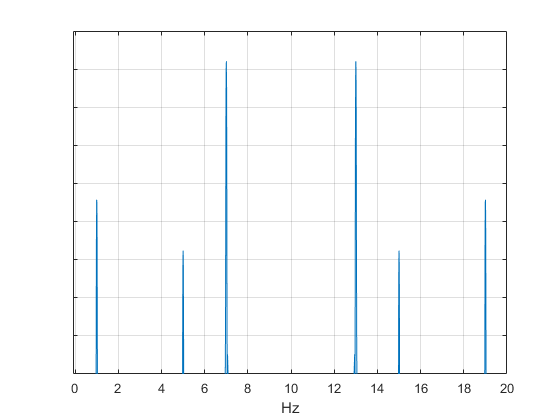
Here is a function adc_dac_harm2.m that plots the spectrum over the 1st and 2nd Nyquist zones. For f0 = 7, fs= 20 and p=5, the function call is as shown. The resulting spectrum plot is shown below.
adc_dac_harm2(7,20,12,5)
But note you get the exact same spectrum for function call
adc_dac_harm2(13,20,12,5)
For this case, f0 = 13 Hz, which is in the 2nd Nyquist zone, and has an alias at 7 Hz. You also get the same result for f0= 27 Hz in the 3rd Nyquist zone, 33 Hz in the 4th Nyquist zone, etc.
% adc_dac_harm2.m   2/15/23 Neil Robertson
% Data converter spectrum due to nonlinearity and aliasing for
% a quantized sinewave input.
%  ***** Plot spectrum over 0 to fs
% f0 = sine frequency (Hz)
% fs = sample frequency (Hz)
% nbits = data converter effective number of bits
% p = exponent of nonlinearity.  p is an integer > 1.
% c (optional) = coefficient of nonlinear term.  default = -.05
function adc_dac_harm2(f0,fs,nbits,p,c)
if nargin == 4
    c= -.05;                            % default value
end
Ts=1/fs;                                % s sample time
N= 2048;                                % number of time samples
n= 0:N-1;                               % time index
x= sin(2*pi*f0*n*Ts);                   % sinewave (simplified NCO)
x= round(x*2^(nbits-1))/2^(nbits-1);    % quantized sinewave
y= x + c*x.^p;                        % apply nonlinearity
nfft= N;                                % number of FFT freq. samples
window= kaiser(N,9);                    % window function
yw= y.*window';
[Y,f]= freqz(yw,1,nfft,'whole',fs);     % DFT using freqz
YdB= 20*log10(abs(Y));
plot(f,YdB),grid
axis([-fs/200 fs -30 60])
xlabel('Hz'),yticklabels(' ')
I hope I understood your question correctly. Let me know if not.
regards,
Neil
To post reply to a comment, click on the 'reply' button attached to each comment. To post a new comment (not a reply to a comment) check out the 'Write a Comment' tab at the top of the comments.
Please login (on the right) if you already have an account on this platform.
Otherwise, please use this form to register (free) an join one of the largest online community for Electrical/Embedded/DSP/FPGA/ML engineers:


