


A DSP Quiz Question
Here's a DSP Quiz Question that I hope you find mildly interesting
BACKGROUND
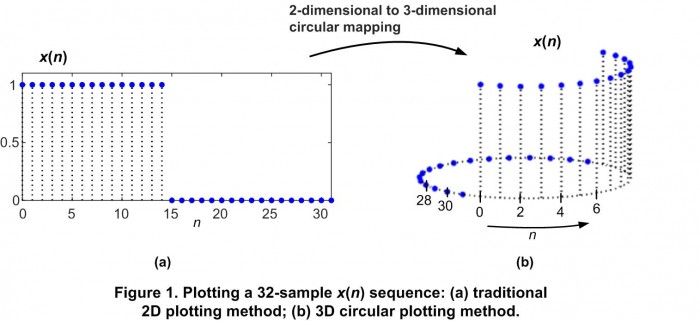
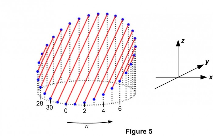
Due to the periodic natures an N-point discrete Fourier transform (DFT) sequence and that sequence’s inverse DFT, it is occasionally reasonable to graphically plot either of those sequences as a 3-dimensional (3D) circular plot. For example, Figure 1(a) shows a length-32 x(n) sequence with its 3D circular plot given in Figure 1(b).
HERE'S THE QUIZ QUESTION:
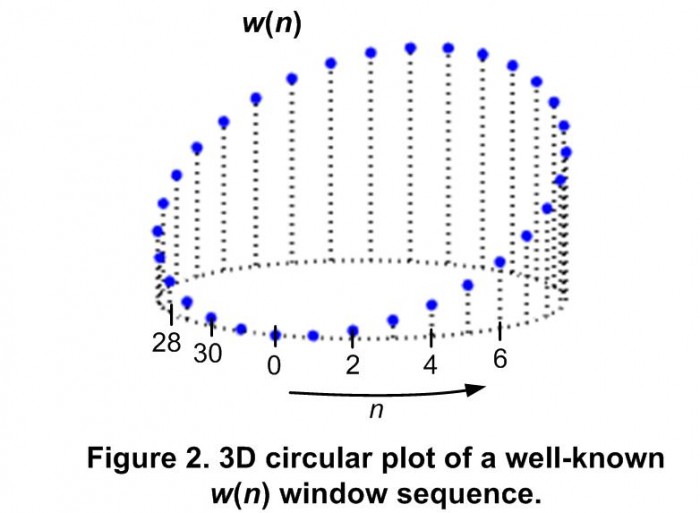
The Quiz Question is: What’s the name of that well-known Figure 2 window sequence?
......
Scroll down to see the question’s answer....
...
...
...
...
...
ANSWER:
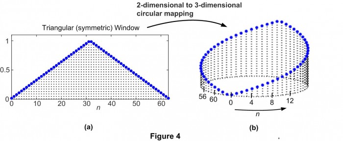
When I first saw what appeared to be a linearly increasing nature of the circular Figure 2 sequence I hastily assumed it was a 3D plot of a triangular window sequence. I was wrong! The Figure 2 sequence is a 32-point hanning (hann) window sequence defined by:$$w(n) = 0.5 -0.5*cos(2*\pi*n/N)$$
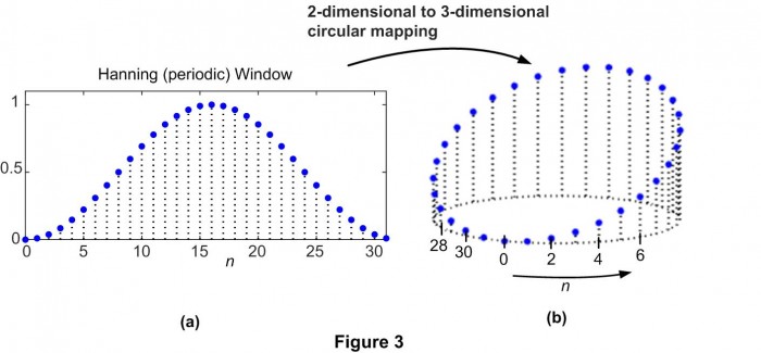
as shown in Figure 3.
TRIVIA:
Postscript:
The paper that caused me to think about all of this is:
Duncan, Andrew, “The Analytic Impulse”, J. Audio Eng. Soc., Vol. 36, No. 5, May 1988. Available online: http://andrewduncan.net/air/
(An incorrect hanning window equation was used in this paper’s Figure 16.)
- Comments
- Write a Comment Select to add a comment

I think it is quite clear that it has to be a closed cosine function, since this is exactly that we have to program into CNC-machines to get the classic oblique section of pipes cut out to get them put together in 90 degrees. (Sometimes the practical training in metal construction that we "old" electrical engineers had to do does help a bit :-)
BTW: Why is the window function still called "hanning"? After all, his name was Mr. "von Hann". (also a possible QUIZ-question.

Regarding the window name "hanning", I don't have a good answer for you. Hanning was the window name I learned decades ago when I first started to study DSP. For many years the MATLAB software had a 'hanning()" command, but sometime after 1997 they changed that command to 'hann()'. Perhaps the DSP pioneers Charles (Charlie) Rader and fred harris, who frequent this web site, could shed some light on the origin of the misnomer "hanning".
fred harris used the term "hanning" in his seminal 'windows' paper ("On the Use of Windows for Harmonic Analysis with the Discrete Fourier Transform") in 1978 but later used the term "hann" in his 2004 "Multirate Signal Processing for Communication Systems" textbook.
Hi,
I also don't understand why the Hann window (proposed by Austrian meterologist Julius von Hann) is still and so often erroneously called "Hanning" window. (I was even taught the name "von-Hann window".) The origin of this confusion is the article The Measurement of Power Spectra from the Point of View of Communications Engineering — Part I by Blackman and Tukey from 1958, where, on page 200, the "use" of this window is denoted as "hanning" (note the lowercase spelling). In an analog fashion, the term "hamming" is used for the process of applying the Hamming window, increasing the confusion even more, since the Hamming window was proposed by the American mathematician Richard Hamming.
Maybe, 64 years later, we are on the way of removing this confusion once and for all. Let's simply continue to use the correct names and others will follow. I guess...
Yeah, good idea. We have to inform the Python guys too, to do that - see posting of dec 21 below:
"z = np.hanning(n)"

Hi Rick,
I worked out what the signal equation would be if the sample values were equal to the y coordinate of that the sample. Taking the origin as the location of n=0 and y axis as being along the line between sample n=0 and n=16. (also taking the radius of the circle to be 1)
My result was x[n] = 1-cos(n/11.25)
This I believe is essentially equivalent the the answer given in the post.
Thanks for the quiz,
Kevin
Hi kevin_keegan. You're causing me to think further about my blog's topic. Your equation 'x[n] = 1-cos(n/11.25)' is interesting. I wonder, from where did the number 11.25 come?
Hi,
360(deg)/32(samples around the circle) = 11.25
I was using degrees not radians, which in retrospect might have been confusing.
Hi kevin_keegan. Yep, you're right because cos(x) functions are based on the notion that angle 'x' is measured in radians (not degrees). So your equation should be:
x[n] = 1-cos(2*pi*n/32).
These are very nice 3D plots, I tried to make them myself in matlab but don't succeed in getting the vertical lines from (x,y,0) to (x,y,z). Is there a way to achieve this in matlab? This is what I currently have:
r=1;
n=32;
teta=-pi:2*pi/(n-1):pi;
x=r*cos(teta);
y=r*sin(teta);
z=hann(n);
plot3(x,y,z,'x')
Hi bertramaets.
Change your 'plot3()' command to:
plot3(x,y,z,'bo','markersize',3,'MarkerFaceColor','b')
and then follow that command with:
for K = 1:n % Plot vertical lines & dots
hold on
plot3([x(K),x(K)],[y(K),y(K)],[0,z(K)],':k', 'linewidth', 1.25)
hold off
end

I wondered Python equivalent, this is quick sketch code;
import numpy as np
import matplotlib.pyplot as plt
r = 1
n = 32
teta = np.linspace(0, 2*np.pi, n)
x = r * np.cos(teta)
y = r * np.sin(teta)
z = np.hanning(n)
#plt.plot3(x,y,z,'bo','markersize',3,'MarkerFaceColor','b')


fig, ax = plt.subplots(subplot_kw=dict(projection='3d'), figsize=(12,12))
ax.stem(x, y, z)
#ax.set(xlabel='x', ylabel='y', zlabel='z')
ax.text(1, 0 , -0.05, '0', fontsize=15)
ax.text(x[1], y[1], -0.05, '1', fontsize=15)
ax.text(x[2], y[2], -0.05, '2', fontsize=15)
ax.text(x[~1], y[~1], -0.05, f'{n-1}', fontsize=15)
ax.text(x[~2], y[~2], -0.05, f'{n-2}', fontsize=15)
ax.axis('off')
ax.set_xticks([])
ax.set_yticks([])
ax.set_zticks([])
ax.view_init(5, 20)


plt.savefig('hann.png')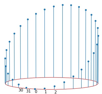
Thanks a lot Rick for these commands which plot the expected !
To post reply to a comment, click on the 'reply' button attached to each comment. To post a new comment (not a reply to a comment) check out the 'Write a Comment' tab at the top of the comments.
Please login (on the right) if you already have an account on this platform.
Otherwise, please use this form to register (free) an join one of the largest online community for Electrical/Embedded/DSP/FPGA/ML engineers:


