Learn About Transmission Lines Using a Discrete-Time Model

• Matlab
• Tutorials

We don’t often think about signal transmission lines, but we use them every day.  Familiar examples are coaxial cable, Ethernet cable, and Universal Serial Bus (USB).  Like it or not, high-speed clock and signal traces on printed-circuit boards are also transmission lines.

While modeling transmission lines is in general a complex undertaking, it is surprisingly simple to model a lossless, uniform line with resistive terminations by using a discrete-time approach.  A discrete-time model easily computes both time and frequency responses, and serves as a good learning tool.  In this post, I provide discrete-time Matlab functions tline and wave_movie, and use them to model lossless uniform transmission lines (note these simple models can approximate lossy transmission lines only if they are short).  Before delving into transmission line math, let’s look at a practical case:  a pulse on a printed-circuit board (PCB) trace.

Example 1.  Pulse on a microstrip line

A microstrip transmission line consists of a trace on the top layer of a PCB with a ground plane on a lower layer.  Figure 1 shows a cross section of a microstrip line of length L = 10 cm, fed by a digital driver and terminated in a buffer.  We will neglect the buffer’s input capacitance, and assume a resistive load as shown.  We also assume no discontinuities along the line, such as sharp bends or vias.  Let the line have a propagation velocity of 0.55 times the speed of light and a characteristic impedance Z₀ of 75 ohms.  Z₀ can be calculated from the line’s dimensions and substrate properties [1].  There are also microstrip impedance calculators available on the web [2].

Now suppose the total source resistance R_S is 20 ohms and the load resistance R_L is 50 k ohms, and let the input signal V_S be a pulse with sample time T_s = 38 ps, as defined in the following Matlab code.  The output V_L of the line is computed by the function tline (Appendix A of the PDF version).  Figure 2 shows the pulse input V_S (top) and the output V_L (middle).

    L= 0.1;                % m length of line (10 cm = 3.94 inch)
    v_rel= 0.55;           %    approx relative velocity, FR-4 microstrip
    Z0= 75;                % ohms line characteristic impedance
    RS= 20;                % ohms source resistance
    RL= 50000;             % ohms load resistance
    Ts= 38E-12;            % s sample time of VS
    VS= [zeros(1,8) ones(1,256) zeros(1,256)];    % pulse
    VL= tline(VS,L,v_rel,Z0,RS,RL,Ts);
    n= 0:length(VL)-1;      %  time index        
    t= n*Ts*1e9;            % ns

The ringing of the output is due to reflected waves traveling back and forth on the line.  After the initial rising edge, the output changes each time the reflected pulse edge makes a trip from load to source and back to load.  (Note a real-world signal would not have such sharp edges, for two reasons: first, the input signal would have a finite bandwidth; and second, the microstrip line would have frequency-dependent loss).  To reduce the reflections, we can adjust the source resistance to approximately Z₀.  For example, if R_S = 80 ohms, we get the output shown in the bottom plot of Figure 2.  The response is improved because the matching source resistance absorbs the wave reflected from the load.  Such an arrangement is called a singly-terminated microstrip line.

We can also view an animation of the waves travelling on the microstrip line using wave_movie (Appendix B of the PDF version).  Here is the Matlab code for a movie of a transmission line with step input:

    Z0= 75;                    % ohms line characteristic impedance
    RS= 20; RL= 50000;         % ohms source and load resistance
    VS= [zeros(1,24) ones(1,180)];    % step input
    wave_movie(VS,Z0,RS,RL);

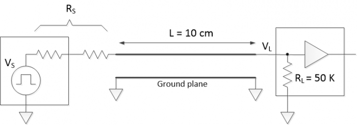
Figure 1.  Microstrip transmission line example.

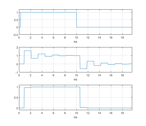
Figure 2.  Microstrip Transmission line signals using function tline.

Top:  input V_S.   Middle: output V_L for R_S = 20 ohms.   Bottom: output V_L for R_S = 80 ohms.

A Very Brief Summary of the Wave Equation for Transmission Lines

In conventional circuit analysis, we assume signals on a wire or printed-circuit trace are functions solely of time.  But at high frequencies, signals are a function of time and position, and a length of wire or a trace becomes a transmission line.  The lossless transmission line model of Figure 3 represents a small length of line dz by a series inductor and shunt capacitor.  L and C have dimensions of inductance per length and capacitance per length; their values depend on the geometry of the line [3].  Voltage on the line obeys the one-dimensional wave equation [4]:

$$ \frac{\delta^2 V}{\delta z^2}= \frac{1}{v^2} \frac{\delta^2 V}{\delta t^2} \qquad (1) $$

where

$$ v= \frac{1}{\sqrt{LC}} \qquad (2) $$

The solution of Equation 1 is any function of the variable t – z/v:

$$ V(t,z)=F(t- \frac{z}{v}) \qquad (3) $$

This equation represents a wave on the transmission line, traveling at velocity v.  For example, suppose a pulse wave travels on a lossless transmission line with v = .8c, where c is the speed of light (3E8 m/s).  Then, if we measure voltage versus z, the result might look something like Figure 4, where we show the relative location of V(z) at three different times: as shown, the pulse wave travels in the positive z direction vs. time.  The full solution of Equation 1 includes a wave traveling in the negative direction:

$$ V(t,z)=F_1(t- \frac{z}{v}) + F_2(t+ \frac{z}{v})  \qquad (4) $$

We can write this as:

$$ V(t,z)=  V_+\; + \; V_- \qquad (5) $$

Where V₊ is a wave traveling in the positive direction, and V_- is a wave traveling in the negative direction.

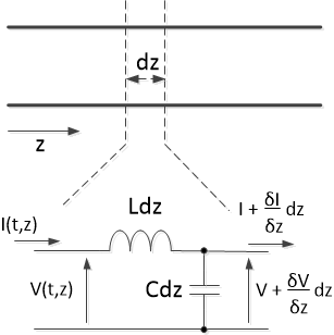
Figure 3.  Lossless transmission line model.

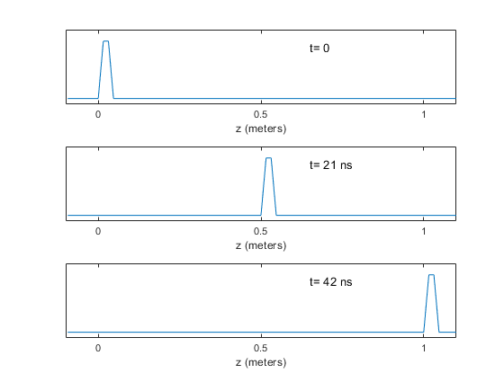
Figure 4.  Pulse wave amplitude vs. distance and time on a lossless transmission line.

top: t = 0.   middle: t= 21 ns.   bottom: t= 42 ns.

Characteristic Impedance and Reflection Coefficient [5]

The ratio of voltage to current for either the positive-travelling or negative-travelling wave is a constant of the transmission line called the characteristic impedance Z₀.  For a lossless line it is given by:

$$ Z_0= \sqrt{\frac{L}{C}} \qquad (6) $$

Although it is called an impedance, Z₀ is real-valued.  If the load resistance at the end of the line is not equal to Z₀, a reflected wave V_- is produced, as shown in Figure 5.  The ratio V_-/V₊ is called the reflection coefficient, and for pure-resistive load it is given by:

$$ \frac{V_-}{V_+} = \rho= \frac{R_L -Z_0}{R_L +Z_0} \qquad(7) $$

For R_L = Z₀, there is no reflection, and ρ = 0.  When R_L is greater than Z₀, ρ is positive.  When R_L is less than Z₀, ρ is negative, and the sign of V_- is the inverse of the sign of V₊.  For R_L = 0, ρ = -1, and for R_L >> Z₀, ρ approaches + 1.  Thus, the possible range of ρ is -1 to +1.

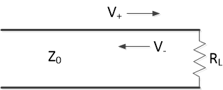
Figure 5.  Reflection on a transmission line with resistive load.

Lossless Transmission Line with Sinusoidal Voltages [6]

Let a sinusoidal voltage be represented by:

$$ V= Ae^{j\omega t} \qquad(8) $$

If we apply this signal to a lossless transmission line, we obtain a positively travelling wave (see Equation 3):

$$ V= V_+ e^{j\omega (t-z/v)} \qquad(9) $$

Allowing for a negatively travelling wave as well, the total voltage is:

$$ V= e^{j\omega t}(V_+ e^{-j\omega z/v} + V_-  e^{j\omega z/v} ) \qquad(10) $$

We can shorten this to:

$$ V= e^{j\omega t}(V_+ e^{-j\beta z} + V_-  e^{j\beta z} ) \qquad(11) $$

where β is called the phase constant:

$$ \beta= \frac{\omega}{v} \qquad(12) $$

Phase constant β represents the phase at z relative to the phase at z = 0.  The phase at two values of z is equal when β*Δz = 2πk.  For k = 1, the value of Δz is called the wavelength λ. Thus:

$$ \beta \lambda = 2\pi $$

and

$$ \beta = \frac{2\pi}{\lambda} \qquad(13) $$

Using Equation 12, we can also write:

$$ \lambda = \frac{v}{f} \qquad(14) $$

The reflection coefficient for a resistive load was given by Equation 7.  For general source or load impedances, the reflection coefficients are:

$$  \rho_S= \frac{Z_S -Z_0}{Z_S +Z_0} \qquad  \rho_L= \frac{Z_L -Z_0}{Z_L +Z_0} \qquad (15) $$

Note ρ is in general complex and |ρ| <=1.

A Discrete-Time Lossless Transmission Line Model

Now let’s create the discrete-time model.  The model will consider only resistive source and load.  Figure 6a shows a transmission line with characteristic impedance Z₀ and length L, connected between source R_S and load R_L.  The reflection coefficients due to the source and load terminations are shown.  A wave travelling in either direction on the line undergoes a delay over the line’s length of:

$$ D= \frac{L}{v} \qquad(16) $$

where v is propagation velocity.  We want to replace this delay with a discrete-time delay of M samples.  Given sample time T_s, we have:

$$ M= round(\frac{D}{T_s}) \qquad(17) $$

We need the delay to operate on both the positive and negative travelling waves, which is achieved using the block diagram of Figure 6b.  (Here z^-M represents a delay of M samples, not distance on the line!)  The real gains ρ_S and ρ_L account for the reflections at source and load.  The gain K takes into account the gain of the cascade of source, transmission line, and load.  Note that this block diagram models the signals at the ends of the transmission line, but not along the length of the line.  We’ll consider the latter case later in this article.

The z-domain transfer function of the block diagram in Figure 6b is:

$$ H(z)= \frac{V_L}{V_S}= K \frac{z^{-M}}{1- \rho_S \rho_L z^{-M} z^{-M}} $$

$$ H(z)= K \frac{z^{-M}}{1- \rho_S \rho_L z^{-2M}} \qquad(18) $$

where

$$ K= \frac{R_S}{(R_S+Z_0)} \frac{2R_L}{(R_L+Z_0)} $$

The expression for K was developed using a circuit model: see Appendix C of the PDF version.  We can rewrite Equation 18 using IIR filter coefficients:

$$ H(z)= K \frac{b_Mz^{-M}}{1+ a_{2M} z^{-2M}} \qquad(19) $$

where

$$ b_M= 1 \quad and \quad a_{2M}= -\rho_S \rho_L $$

The time response of the transmission line is then given by the difference equation:

$$ y(n)= Kb_Mx(n-M) - a_{2M}y(n-2M) \qquad (20) $$

Where x = V_S and y = V_L.  This simple result applies for any signal waveform, provided that source and load are resistive.  Equation 20 is implemented by the Matlab function tline (See Appendix A of the PDF version).  We used tline in Example 1.

For the case of general source and load impedance, the reflection coefficients are complex functions of frequency.  This case requires a more sophisticated model than the one presented here.  An expression for H(jω) of a lossless transmission line for general source and load impedances is derived in Appendix C of the PDF version (Equation C10).

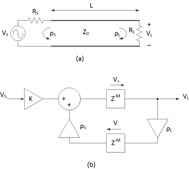
Figure 6. a) Lossless transmission line, showing source and load reflection coefficients.

               b) Lossless transmission line discrete-time model.

Example 2.  Frequency Response of a Lossless Transmission Line

In this example, we’ll compute the frequency response of the lossless transmission line shown in Figure 6a for several values of R_S and R_L  (we won't use tline.m here).  Let the transmission line have the following properties:

Z₀ = 75 ohms

L = 1 m

v_rel = 0.8 (velocity relative to the speed of light c = 3E8 m/s)

v= v_rel*c

Rather than compute M based on T_s (Equations 16 and 17), we’ll use M = 8 samples for the model’s delay and compute the resulting T_s.  Given line delay D = L/v and T_s = D/M, this value of M results in T_s of 521 ps, or f_s of 1.92 GHz.  The following Matlab code computes the coefficients of Equation 19, then finds the frequency response using freqz.  We’ll scale the gain such that the transfer function is H(z) = V_L/(V_S/2), where V_S/2 is the gain when R_L = R_S = Z₀.

    L= 1;                % m length of line
    v_rel= 0.8;          %   velocity relative to speed of light
    c= 3E8;              % m/s speed of light
    v= v_rel*c;          % m/s propagation velocity
    D= L/v;              % s delay of line
    M= 8;                % samples delay of line
    Ts= D/M;             % s sample time
    fs= 1/Ts             % Hz sample frequency
    Z0= 75;              % ohms line characteristic impedance
    RS= 75; RL= 75;      % ohms source and load resistance
    Krel= 2* Z0/(RS+ Z0) * 2*RL/(RL+ Z0);      % gain const. relative to VS/2
    rho_S= (RS - Z0)/(RS + Z0);                % input reflection coeff
    rho_L= (RL - Z0)/(RL + Z0);                % output reflection coeff
    b= [zeros(1,M) 1];                         % feed forward coeffs
    a= [1 zeros(1,2*M-1) -rho_S*rho_L];        % feedback coeffs
    [h,f]= freqz(Krel*b,a,256,fs/1e6);
    H= 20*log10(abs(h));

Case I:  R_S = R_L = Z₀ = 75 ohms.  The response is plotted in the top of Figure 7.For this case, there are no reflections, and the response is flat with gain of 0 dB (The response of a lossy line would roll-off vs. frequency, in this and the following cases).

Case II:  R_S = 150 ohms, R_L = 37.5 ohms.  The response is plotted in the middle of Figure 7.  Mismatches at both source and load cause ripple of roughly 2 dB in the response.

Case III:  R_S = R_L = 5 ohms.  The response is plotted in the bottom of Figure 7.  For this case, the product of ρ_L and ρ_S is 0.766, and we see resonances at 120 MHz and its harmonics.  As ρ_L ρ_S approaches 1, |H(z)|/K approaches the inverse of a comb filter response.  We’ll examine this case further in Example 3.

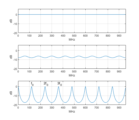
Figure 7.  Lossless line frequency response magnitude for Example 2, Z₀ = 75 ohms.

   Top: R_S = R_L = Z₀    Middle: R_S = 150 ohms, R_L = 37.5 ohms.   Bottom: R_S = R_L = 5 ohms.

Example 3.  Standing Waves in a Resonator

In Example 2, we found the frequency response of a 75-ohm transmission line with RS = RL = 5 ohms (See circuit diagram in Figure 8).  The response was resonant at 120 MHz and harmonics.  The longest wavelength resonance occurs when wavelength is twice the length of the line:

$$ \lambda_0= 2L \qquad (21) $$

Thus, from Equation 14, the lowest resonant frequency f₀ is:

$$ f_0= \frac{v}{2L} \qquad (22) $$

In this case, f₀ = (0.8*3E8)/2 = 120 MHz.

Our transmission line model of Figure 6b represents the line with M time samples.  This corresponds to a sample spacing in distance of L/M.  By summing the positive and negative traveling waves, we can plot the line voltage vs. distance and time.  The function wave_movie (Appendix B of the PDF version) plots an animation of the voltage on the line, using M= 16.  Here is Matlab code to call wave_movie for a sine at 120 MHz.  Note that the code must calculate the sine’s sample time T_s based on L, v, and M.

    L= 1;                      % m length of line
    v_rel= 0.8;                %  velocity relative to speed of light
    M= 16;                     %  samples delay of t-line
    v= v_rel*3E8;              % m/s propagation velocity
    D= L/v;                    % s delay of line
    Ts= D/M;                   % s sample time
    % sinewave
    fc= 120E6;                 % Hz sine freq
    N= 300;                    %  number of time samples
    n= 0:N-1;                  %  time index
    VS= sin(2*pi*fc*n*Ts);     %  input signal
    Z0= 75;                    % ohms line characteristic impedance
    RS= 5; RL= 5;              % ohms source and load resistances
    wave_movie(VS,Z0,RS,RL);

A cumulative plot of the resulting animation is shown in Figure 9 (top).  Each curve approximates 1/2 cycle of a sinewave at a given instant in time.  Thus, wavelength is 2L, which is consistent with Equation 21.  Although V₊ and V_- move at velocity v, their sum along the line does not travel, producing a standing wave.  Looking at harmonics of the 120 MHz fundamental frequency: for f_c = 240 MHz, each curve approximates a full cycle of a sinewave (Figure 9, middle), and 320 MHz gives 1.5 cycles (bottom).  The amplitude of V_S is 1 V peak, while the maximum amplitude of the standing waves is about 7.5 V.  For frequencies not close to multiples of 120 MHz, the amplitude is much lower, as you would expect from the frequency response of Figure 7 (bottom).  The standing waves are analogous to the waves on the plucked string of a guitar (but at much higher frequencies!)[7].  For a guitar, the fundamental and harmonics are present simultaneously on the string.

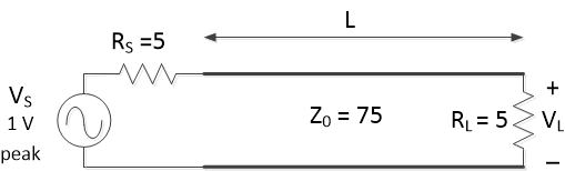
Figure 8.  Transmission line acting as a resonator.

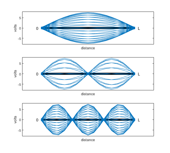
Figure 9.  Standing waves in a resonator:  cumulative plots from wave_movie.m

       Top:  f_c = 120 MHz.   Middle:  f_c = 240 MHz.   Bottom:  f_c = 360 MHz.

For Appendices, see the PDF version of this article.

References

1.  Ludwig, Reinhold and Bogdanov, Gene, RF Circuit Design, 2^nd Ed., Pearson, 2009, section 2.8.

2.  Campbell, David, Microstrip Calculator,

https://www.microwaves101.com/calculators/1201-microstrip-calculator

3.  Ludwig, sections 2.2 - 2.6.

4.  Ramo, Simon; Whinnery, John; and Van Duzer, Theodore, Fields and Waves in Communication Electronics, Wiley, 1965, section 1.14.

5.  Ramo, sections 1.15 – 1.16.

6.  Ramo, section 1.18.

7.  Peterson, Mark R., “Musical Analysis and Synthesis in Matlab”, College Mathematics Journal, Vol. 35, No. 5, Nov. 2004, https://amath.colorado.edu/pub/matlab/music/Petersen04CMJ.pdf

8.  Ludwig, sections 4.1 – 4.2.

 January, 2022        Neil Robertson

Sign in