


Time-Varying Two-Pole Filters
It is quite common to want to vary the resonance frequency of a resonator in real time. This is a special case of a tunable filter. In the pre-digital days of analog synthesizers, filter modules were tuned by means of control voltages, and were thus called voltage-controlled filters (VCF). In the digital domain, control voltages are replaced by time-varying filter coefficients. In the time-varying case, the choice of filter structure has a profound effect on how the filter characteristics vary with respect to coefficient variations. In this section, we will take a look at the time-varying two-pole resonator.
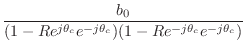
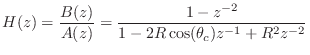
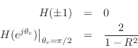
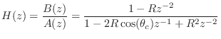
Evaluating the transfer function of the two-pole resonator
(Eq.![]() (B.1)) at the point
(B.1)) at the point
![]() on the unit circle
(the filter's resonance frequency
on the unit circle
(the filter's resonance frequency
![]() ) yields a gain at resonance equal to
) yields a gain at resonance equal to
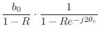
For simplicity, let
Since
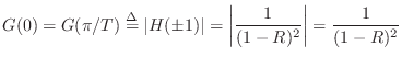
An important fact we can now see is that the gain at resonance depends markedly on the resonance frequency. In particular, the ratio of the two cases just analyzed is

Note that the ratio of the dc resonance gain to the ![]() resonance
gain is unbounded! The sharper the resonance (the closer
resonance
gain is unbounded! The sharper the resonance (the closer ![]() is to 1), the greater the disparity in the gain.
is to 1), the greater the disparity in the gain.
Figure B.17 illustrates a number of resonator frequency responses
for the case ![]() . (Resonators in practice may use values of
. (Resonators in practice may use values of ![]() even closer to 1 than this--even the case
even closer to 1 than this--even the case ![]() is used for making
recursive digital sinusoidal oscillators [90].) For
resonator tunings at dc and
is used for making
recursive digital sinusoidal oscillators [90].) For
resonator tunings at dc and ![]() , we predict the resonance gain to
be
, we predict the resonance gain to
be
![]() dB, and this is what we see in the plot.
When the resonance is tuned to
dB, and this is what we see in the plot.
When the resonance is tuned to ![]() , the gain drops well below 40
dB. Clearly, we will need to compensate this gain variation when
trying to use the two-pole digital resonator as a tunable filter.
, the gain drops well below 40
dB. Clearly, we will need to compensate this gain variation when
trying to use the two-pole digital resonator as a tunable filter.
![\includegraphics[width=\twidth ]{eps/resgain}](http://www.dsprelated.com/josimages_new/filters/img1506.png) |
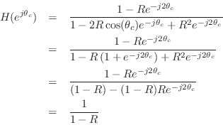
Figure B.18 shows the same type of plot for the complex
one-pole resonator
![]() , for
, for ![]() and
10 values of
and
10 values of ![]() . In this case, we expect the frequency
response evaluated at the center frequency to be
. In this case, we expect the frequency
response evaluated at the center frequency to be
![]() . Thus, the gain at
resonance for the plotted example is
. Thus, the gain at
resonance for the plotted example is
![]() db for all
tunings. Furthermore, for the complex resonator, the resonance gain
is also exactly equal to the peak gain.
db for all
tunings. Furthermore, for the complex resonator, the resonance gain
is also exactly equal to the peak gain.
![\includegraphics[width=\twidth ]{eps/cresgain}](http://www.dsprelated.com/josimages_new/filters/img1509.png) |
Normalizing Two-Pole Filter Gain at Resonance
The question we now pose is how to best compensate the tunable
two-pole resonator of §B.1.3 so that its peak gain is the same for
all tunings. Looking at Fig.B.17, and remembering the graphical
method for determining the amplitude response,B.6 it is intuitively
clear that we can help matters by adding two zeros to the
filter, one near dc and the other near ![]() . A zero exactly at dc
is provided by the term
. A zero exactly at dc
is provided by the term
![]() in the transfer function numerator.
Similarly, a zero at half the sampling rate is provided by the term
in the transfer function numerator.
Similarly, a zero at half the sampling rate is provided by the term
![]() in the numerator. The series combination of both zeros
gives the numerator
in the numerator. The series combination of both zeros
gives the numerator
![]() . The complete
second-order transfer function then becomes
. The complete
second-order transfer function then becomes
Checking the gain for the case
which is better behaved, but now the response falls to zero at dc and
![]() rather than being heavily boosted, as we found in
Eq.
rather than being heavily boosted, as we found in
Eq.![]() (B.12).
(B.12).
Constant Resonance Gain
It turns out it is possible to normalize exactly the
resonance gain of the second-order resonator tuned by a
single coefficient [89]. This is accomplished by
placing the two zeros at
![]() , where
, where ![]() is the radius of
the complex-conjugate pole pair . The transfer function numerator
becomes
is the radius of
the complex-conjugate pole pair . The transfer function numerator
becomes
![]() , yielding
the total transfer function
, yielding
the total transfer function
Thus, the gain at resonance is ![]() for all resonance tunings
for all resonance tunings ![]() .
.
Figure B.19 shows a family of amplitude responses for the
constant resonance-gain two-pole, for various values of ![]() and
and
![]() . We see an excellent improvement in the regularity of the
amplitude response as a function of tuning.
. We see an excellent improvement in the regularity of the
amplitude response as a function of tuning.
![\includegraphics[width=\twidth ]{eps/cgresgain}](http://www.dsprelated.com/josimages_new/filters/img1523.png) |
Peak Gain Versus Resonance Gain
While the constant resonance-gain filter is very well behaved, it is
not ideal, because, while the resonance gain is perfectly
normalized, the peak gain is not. The amplitude-response peak
does not occur exactly at the resonance frequencies
![]() except for the special cases
except for the special cases
![]() ,
, ![]() ,
and
,
and ![]() . At other resonance frequencies, the peak due to one pole
is shifted by the presence of the other pole.
When
. At other resonance frequencies, the peak due to one pole
is shifted by the presence of the other pole.
When ![]() is close to 1, the shifting can be negligible, but in more
damped resonators, e.g., when
is close to 1, the shifting can be negligible, but in more
damped resonators, e.g., when ![]() , there can be a significant
difference between the gain at resonance and the true peak gain.
, there can be a significant
difference between the gain at resonance and the true peak gain.
Figure B.20 shows a family of amplitude responses for the
constant resonance-gain two-pole, for various values of ![]() and
and
![]() . We see that while the gain at resonance is exactly the same
in all cases, the actual peak gain varies somewhat, especially
near dc and
. We see that while the gain at resonance is exactly the same
in all cases, the actual peak gain varies somewhat, especially
near dc and ![]() when the two poles come closest together. A more
pronounced variation in peak gain can be seen in
Fig.B.21, for which the pole radii have been reduced
to
when the two poles come closest together. A more
pronounced variation in peak gain can be seen in
Fig.B.21, for which the pole radii have been reduced
to ![]() .
.
![\includegraphics[width=\twidth ]{eps/cgresgaindamped}](http://www.dsprelated.com/josimages_new/filters/img1526.png) |
![\includegraphics[width=\twidth ]{eps/cgresgaindampedp5}](http://www.dsprelated.com/josimages_new/filters/img1527.png) |
Constant Peak-Gain Resonator
It is surprisingly easy to normalize exactly the peak gain in a second-order resonator tuned by a single coefficient [94]. The filter structure that accomplishes this is the one we already considered in §B.6.1:
That is, the two-pole resonator normalized by zeros at
Real-time audio ``plugins'' based on the constant-peak-gain resonator are developed in Appendix K.
The peak gain is ![]() , so multiplying the transfer function by
, so multiplying the transfer function by
![]() normalizes the peak gain to one for all tunings. It can
also be shown [94] that the peak gain coincides with the
variance gain when the resonator is driven by white noise. That
is, if the variance of the driving noise is
normalizes the peak gain to one for all tunings. It can
also be shown [94] that the peak gain coincides with the
variance gain when the resonator is driven by white noise. That
is, if the variance of the driving noise is ![]() , the variance
of the noise at the resonator output is
, the variance
of the noise at the resonator output is
![]() .
Therefore, scaling the resonator input by
.
Therefore, scaling the resonator input by
![]() will
normalize the resonator such that the output signal power equals the
input signal power when the input signal is white noise.
will
normalize the resonator such that the output signal power equals the
input signal power when the input signal is white noise.
Frequency response overlays for the constant-peak-gain resonator are
shown in Fig.B.23 (![]() ), Fig.B.20
(
), Fig.B.20
(![]() ), and Fig.B.21 (
), and Fig.B.21 (![]() ). While the peak
frequency may be far from the resonance tuning in the more heavily
damped examples, the peak gain is always normalized to unity. The
normalized radian frequency
). While the peak
frequency may be far from the resonance tuning in the more heavily
damped examples, the peak gain is always normalized to unity. The
normalized radian frequency
![]() at which the peak gain
occurs is related to the pole angle
at which the peak gain
occurs is related to the pole angle
![]() by
[94]
by
[94]
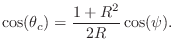
When the right-hand side of the above equation exceeds 1 in magnitude, there is no (real) solution for the pole frequency
![\includegraphics[width=\twidth ]{eps/psivsthetac}](http://www.dsprelated.com/josimages_new/filters/img1543.png)
Thus, ![]() must be close to 1 to obtain a resonant peak near dc (a case
commonly needed in audio work) or half the sampling rate (rarely
needed in practice). When
must be close to 1 to obtain a resonant peak near dc (a case
commonly needed in audio work) or half the sampling rate (rarely
needed in practice). When ![]() is much less than 1, the peak frequency
is much less than 1, the peak frequency
![]() cannot leave a small interval near one-fourth the sampling
rate, as can be seen at the far left in Fig.B.22.
cannot leave a small interval near one-fourth the sampling
rate, as can be seen at the far left in Fig.B.22.
Figure B.22 predicts that for ![]() , the lowest peak-gain
frequency should be around
, the lowest peak-gain
frequency should be around
![]() radian per sample.
Figure B.21 agrees with this prediction.
radian per sample.
Figure B.21 agrees with this prediction.
As Figures B.23 through B.25 show, the peak gain remains
constant even at very low and very high frequencies, to the extent
they are reachable for a given ![]() . The zeros at dc and
. The zeros at dc and ![]() preclude the possibility of peaks at exactly those frequencies, but
for
preclude the possibility of peaks at exactly those frequencies, but
for ![]() near 1, we can get very close to having a peak at dc or
near 1, we can get very close to having a peak at dc or
![]() , as shown in Figures B.19 and B.20.
, as shown in Figures B.19 and B.20.
![\includegraphics[width=\twidth ]{eps/cpgresgain}](http://www.dsprelated.com/josimages_new/filters/img1546.png) |
![\includegraphics[width=\twidth ]{eps/cpgresgaindamped}](http://www.dsprelated.com/josimages_new/filters/img1547.png) |
![\includegraphics[width=\twidth ]{eps/cpgresgaindampedp5}](http://www.dsprelated.com/josimages_new/filters/img1548.png) |
Four-Pole Tunable Lowpass/Bandpass Filters
As a practical note, it is worth mentioning that in popular analog synthesizers (both real and virtualB.7), VCFs are typically fourth order rather than second order as we have studied here. Perhaps the best known VCF is the Moog VCF. The four-pole Moog VCF is configured to be a lowpass filter with an optional resonance near the cut-off frequency. When the resonance is strong, it functions more like a resonator than a lowpass filter. Various methods for digitizing the Moog VCF are described in [95]. It turns out to be nontrivial to preserve all desirable properties of the analog filter (such as frequency response, order, and control structure), when translated to digital form by standard means.
Next Section:
Elementary Filter Problems
Previous Section:
Peaking Equalizers


