


Mass and Dashpot in Series
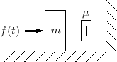
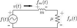
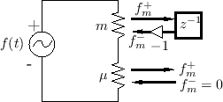
This is our first example illustrating a series connection of wave digital elements. Figure F.26 gives the physical scenario of a simple mass-dashpot system, and Fig.F.27 shows the equivalent circuit. Replacing element voltages and currents in the equivalent circuit by wave variables in an infinitesimal waveguides produces Fig.F.28.
 |
 |
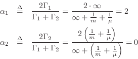
The system can be described as an ideal force source ![]() connected
in parallel with the series connection of mass
connected
in parallel with the series connection of mass ![]() and
dashpot
and
dashpot ![]() .
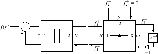
Figure F.29 illustrates the resulting wave digital filter.
Note that the ports are now numbered for reference. Two more symbols
are introduced in this figure: (1) the horizontal line with a dot in
the middle indicating a series adaptor, and (2) the indication of a
reflection-free port on input 1 of the series adaptor (signal
.
Figure F.29 illustrates the resulting wave digital filter.
Note that the ports are now numbered for reference. Two more symbols
are introduced in this figure: (1) the horizontal line with a dot in
the middle indicating a series adaptor, and (2) the indication of a
reflection-free port on input 1 of the series adaptor (signal
![]() ). Recall that a reflection-free port is always necessary
when connecting two adaptors together, to avoid creating a delay-free
loop.
). Recall that a reflection-free port is always necessary
when connecting two adaptors together, to avoid creating a delay-free
loop.
Let's first calculate the impedance ![]() necessary to make input 1 of
the series adaptor reflection free. From Eq.
necessary to make input 1 of
the series adaptor reflection free. From Eq.![]() (F.37), we require
(F.37), we require
The parallel adaptor, viewed alone, is equivalent to a force source
driving impedance ![]() . It is therefore realizable as in
Fig.F.20 with the wave digital spring replaced by the
mass-dashpot assembly in
Fig.F.29. However, we can also carry out a quick analysis
to verify this: The alpha parameters are
. It is therefore realizable as in
Fig.F.20 with the wave digital spring replaced by the
mass-dashpot assembly in
Fig.F.29. However, we can also carry out a quick analysis
to verify this: The alpha parameters are
Therefore, the reflection coefficient seen at port 1 of the parallel
adaptor is
![]() , and the Kelly-Lochbaum scattering
junction depicted in Fig.F.20 is verified.
, and the Kelly-Lochbaum scattering
junction depicted in Fig.F.20 is verified.
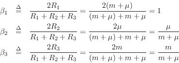
Let's now calculate the internals of the series adaptor in
Fig.F.29. From Eq.![]() (F.26), the beta parameters are
(F.26), the beta parameters are
Following Eq.![]() (F.30), the series adaptor computes
(F.30), the series adaptor computes
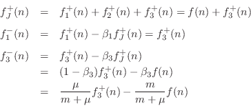
We do not need to explicitly compute
![]() because it goes into a
purely resistive impedance
because it goes into a
purely resistive impedance ![]() and produces no return wave. For the
same reason,
and produces no return wave. For the
same reason,
![]() .
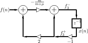
Figure F.30 shows a wave flow diagram of the computations derived,
together with the result of elementary simplifications.
.
Figure F.30 shows a wave flow diagram of the computations derived,
together with the result of elementary simplifications.
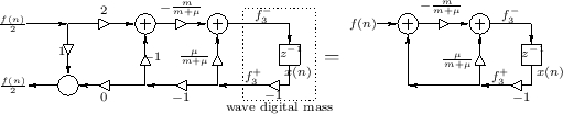 |
Because the difference of the two coefficients in Fig.F.30 is 1, we can easily derive the one-multiply form in Fig.F.31.
Checking the WDF against the Analog Equivalent Circuit
Let's check our result by comparing the transfer function from the input force to the force on the mass in both the discrete- and continuous-time cases.
For the discrete-time case, we have

We now need
![]() .
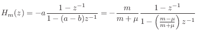
To simplify notation, define the two coefficients as
.
To simplify notation, define the two coefficients as

From Figure F.30, we can write
![\begin{eqnarray*}
F^{-}_3(z) &=& -a\left[F(z)-z^{-1}F^{-}_3(z)\right] + b\left[-...
...\,\,\quad
F^{-}_3(z) &=& -a\frac{F(z)}{1-(a-b)z^{-1}F^{-}_3(z)}
\end{eqnarray*}](http://www.dsprelated.com/josimages_new/pasp/img4987.png)
Thus, the desired transfer function is
We now wish to compare this result to the bilinear transform of the corresponding analog transfer function. From Figure F.27, we can recognize the mass and dashpot as voltage divider:
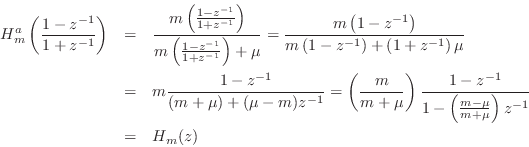
Thus, we have verified that the force transfer-function from the driving force to the mass is identical in the discrete- and continuous-time models, except for the bilinear transform frequency warping in the discrete-time case.
Next Section:
Wave Digital Mass-Spring Oscillator
Previous Section:
Spring and Free Mass


