


Complex Numbers
This chapter introduces complex numbers, beginning with factoring polynomials, and proceeding on to the complex plane and Euler's identity.
Factoring a Polynomial
Remember ``factoring polynomials''? Consider the second-order polynomial
This is a system of two equations in two unknowns. Unfortunately, it is a nonlinear system of two equations in two unknowns.2.1 Nevertheless, because it is so small, the equations are easily solved. In beginning algebra, we did them by hand. However, nowadays we can use a software tool such as Matlab or Octave to solve very large systems of linear equations.
The factored form of this simple example is
The Quadratic Formula
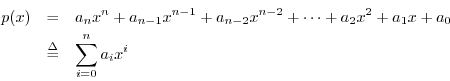
The general second-order (real) polynomial is
where the coefficients
where the magnitude of
Equating coefficients of like powers of
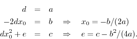
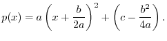
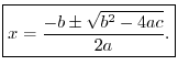
Using these answers, any second-order polynomial
![]() can be rewritten as a scaled, translated parabola
can be rewritten as a scaled, translated parabola
Complex Roots
![\includegraphics[scale=0.5]{eps/parabola}](http://www.dsprelated.com/josimages_new/mdft/img139.png)
As a simple example, let ![]() ,
, ![]() , and
, and ![]() , i.e.,
, i.e.,

It can be checked that all algebraic operations for real
numbers2.2 apply equally well to complex numbers. Both real numbers
and complex numbers are examples of a
mathematical field.2.3 Fields are
closed with respect to multiplication and addition, and all the rules
of algebra we use in manipulating polynomials with real coefficients (and
roots) carry over unchanged to polynomials with complex coefficients and
roots. In fact, the rules of algebra become simpler for complex numbers
because, as discussed in the next section, we can always factor
polynomials completely over the field of complex numbers while we cannot do
this over the reals (as we saw in the example
![]() ).
).
Fundamental Theorem of Algebra
This is a very powerful algebraic tool.2.4 It says that given any polynomial
we can always rewrite it as
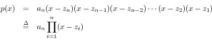
where the points ![]() are the polynomial roots, and they may be real or
complex.
are the polynomial roots, and they may be real or
complex.
Complex Basics
This section introduces various notation and terms associated with complex
numbers. As discussed above, complex numbers arise by introducing
the square-root of ![]() as a primitive new algebraic object among real
numbers and manipulating it symbolically as if it were a real number
itself:
as a primitive new algebraic object among real
numbers and manipulating it symbolically as if it were a real number
itself:
As mentioned above, for any negative number ![]() , we have
, we have
By definition, we have
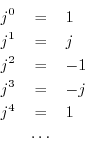
and so on. Thus, the sequence
![]() ,
,
![]() is a
periodic sequence with period
is a
periodic sequence with period ![]() , since
, since
![]() . (We'll
learn later that the sequence
. (We'll
learn later that the sequence ![]() is a sampled complex sinusoid having
frequency equal to one fourth the sampling rate.)
is a sampled complex sinusoid having
frequency equal to one fourth the sampling rate.)
Every complex number ![]() can be written as
can be written as
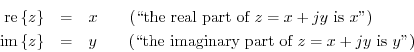
Note that the real numbers are the subset of the complex numbers having
a zero imaginary part (![]() ).
).
The rule for complex multiplication follows directly from the definition
of the imaginary unit ![]() :
:
In some mathematics texts, complex numbers ![]() are defined as ordered pairs
of real numbers
are defined as ordered pairs
of real numbers ![]() , and algebraic operations such as multiplication
are defined more formally as operations on ordered pairs, e.g.,
, and algebraic operations such as multiplication
are defined more formally as operations on ordered pairs, e.g.,
![]() . However, such
formality tends to obscure the underlying simplicity of complex numbers as
a straightforward extension of real numbers to include
. However, such
formality tends to obscure the underlying simplicity of complex numbers as
a straightforward extension of real numbers to include
![]() .
.
It is important to realize that complex numbers can be treated
algebraically just like real numbers. That is, they can be added,
subtracted, multiplied, divided, etc., using exactly the same rules of
algebra (since both real and complex numbers are mathematical
fields). It is often preferable to think of complex numbers as
being the true and proper setting for algebraic operations, with real
numbers being the limited subset for which ![]() .
.
The Complex Plane
![\includegraphics[scale=0.5]{eps/ComplexPlane}](http://www.dsprelated.com/josimages_new/mdft/img176.png)
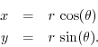
We can plot any complex number ![]() in a plane as an ordered pair
in a plane as an ordered pair
![]() , as shown in Fig.2.2. A complex plane (or
Argand diagram) is any 2D graph in which the horizontal axis is
the real part and the vertical axis is the imaginary
part of a complex number or function. As an example, the number
, as shown in Fig.2.2. A complex plane (or
Argand diagram) is any 2D graph in which the horizontal axis is
the real part and the vertical axis is the imaginary
part of a complex number or function. As an example, the number ![]() has coordinates
has coordinates ![]() in the complex plane while the number
in the complex plane while the number ![]() has
coordinates
has
coordinates ![]() .
.
Plotting ![]() as the point
as the point ![]() in the complex plane can be
viewed as a plot in Cartesian or
rectilinear coordinates. We can
also express complex numbers in terms of polar coordinates as
an ordered pair
in the complex plane can be
viewed as a plot in Cartesian or
rectilinear coordinates. We can
also express complex numbers in terms of polar coordinates as
an ordered pair
![]() , where
, where ![]() is the distance from the
origin
is the distance from the
origin ![]() to the number being plotted, and
to the number being plotted, and ![]() is the angle
of the number relative to the positive real coordinate axis (the line
defined by
is the angle
of the number relative to the positive real coordinate axis (the line
defined by ![]() and
and ![]() ). (See Fig.2.2.)
). (See Fig.2.2.)
Using elementary geometry, it is quick to show that conversion from rectangular to polar coordinates is accomplished by the formulas
where
![]() denotes the arctangent of
denotes the arctangent of ![]() (the angle
(the angle
![]() in radians whose tangent is
in radians whose tangent is
![]() ), taking the
quadrant of the vector
), taking the
quadrant of the vector ![]() into account. We will take
into account. We will take ![]() in
the range
in
the range ![]() to
to ![]() (although we could choose any interval of
length
(although we could choose any interval of
length ![]() radians, such as 0 to
radians, such as 0 to ![]() , etc.).
, etc.).
In Matlab and Octave, atan2(y,x) performs the
``quadrant-sensitive'' arctangent function. On the other hand,
atan(y/x), like the more traditional mathematical notation
![]() does not ``know'' the quadrant of
does not ``know'' the quadrant of ![]() , so it maps
the entire real line to the interval
, so it maps
the entire real line to the interval
![]() . As a specific
example, the angle of the vector
. As a specific
example, the angle of the vector
![]() (in quadrant I) has the
same tangent as the angle of
(in quadrant I) has the
same tangent as the angle of
![]() (in quadrant III).
Similarly,
(in quadrant III).
Similarly,
![]() (quadrant II) yields the same tangent as
(quadrant II) yields the same tangent as
![]() (quadrant IV).
(quadrant IV).
The formula
![]() for converting rectangular
coordinates to radius
for converting rectangular
coordinates to radius ![]() , follows immediately from the
Pythagorean theorem, while the
, follows immediately from the
Pythagorean theorem, while the
![]() follows from the definition of the tangent
function itself.
follows from the definition of the tangent
function itself.
Similarly, conversion from polar to rectangular coordinates is simply
These follow immediately from the definitions of cosine and sine, respectively.
More Notation and Terminology
It's already been mentioned that the rectilinear coordinates of a complex
number ![]() in the complex plane are called the real part and
imaginary part, respectively.
in the complex plane are called the real part and
imaginary part, respectively.
We also have special notation and various names for the polar
coordinates
![]() of a complex number
of a complex number ![]() :
:
The complex conjugate of ![]() is denoted
is denoted
![]() (or
(or ![]() ) and is defined by
) and is defined by

In general, you can always obtain the complex conjugate of any expression
by simply replacing ![]() with
with ![]() . In the complex plane, this is a vertical flip about the real axis; i.e., complex conjugation
replaces each point in the complex plane by its mirror image on the
other side of the
. In the complex plane, this is a vertical flip about the real axis; i.e., complex conjugation
replaces each point in the complex plane by its mirror image on the
other side of the ![]() axis.
axis.
Elementary Relationships
From the above definitions, one can quickly verify
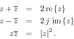
Let's verify the third relationship which states that a complex number multiplied by its conjugate is equal to its magnitude squared:
Euler's Identity
Since
![]() is the algebraic expression of
is the algebraic expression of ![]() in terms of its
rectangular coordinates, the corresponding expression in terms of its polar
coordinates is
in terms of its
rectangular coordinates, the corresponding expression in terms of its polar
coordinates is
There is another, more powerful representation of ![]() in terms of its
polar coordinates. In order to define it, we must introduce Euler's
identity:
in terms of its
polar coordinates. In order to define it, we must introduce Euler's
identity:
A proof of Euler's identity is given in the next chapter. Before, the only algebraic representation of a complex number we had was
A corollary of Euler's identity is obtained by setting
![]() to get
to get
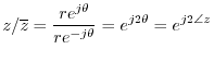
For another example of manipulating the polar form of a complex number,
let's again verify
![]() , as we did above in
Eq.
, as we did above in
Eq.![]() (2.4), but this time using polar form:
(2.4), but this time using polar form:
We can now easily add a fourth line to that set of examples:
Euler's identity can be used to derive formulas for sine and cosine in
terms of
![]() :
:
![\begin{eqnarray*}
e^{j \theta} + \overline{e^{j \theta}}&=&e^{j \theta} + e^{-j ...
...+ \left[\cos(\theta) - j \sin(\theta)\right]\\
&=&2\cos(\theta)
\end{eqnarray*}](http://www.dsprelated.com/josimages_new/mdft/img224.png)
Similarly,
![]() , and
we obtain the following classic identities:
, and
we obtain the following classic identities:

De Moivre's Theorem
As a more complicated example of the value of the polar form, we'll prove De Moivre's theorem:
Conclusion
This chapter has covered just enough about complex numbers to enable us to talk about the discrete Fourier transform.
Manipulations of complex numbers in Matlab and Octave are illustrated in §I.1.
To explore further the mathematics of complex variables, see any textbook such as Churchill [15] or LePage [37]. Topics not covered here, but which are important elsewhere in signal processing, include analytic functions, contour integration, analytic continuation, residue calculus, and conformal mapping.
Complex_Number Problems
See http://ccrma.stanford.edu/~jos/mdftp/Complex_Number_Problems.html
Next Section:
Proof of Euler's Identity
Previous Section:
Introduction to the DFT


