


An Easier Way
We derived the frequency response above using trig identities in order to minimize the mathematical level involved. However, it turns out it is actually easier, though more advanced, to use complex numbers for this purpose. To do this, we need Euler's identity:
where
Complex Sinusoids
Using Euler's identity to represent sinusoids, we have
when time
Any function of the form
![]() or
or
![]() will henceforth be called a complex
sinusoid.2.3 We will
see that it is easier to manipulate both sine and
cosine simultaneously in this form than it is to deal with
either
sine or cosine separately. One may even take the
point of view that
will henceforth be called a complex
sinusoid.2.3 We will
see that it is easier to manipulate both sine and
cosine simultaneously in this form than it is to deal with
either
sine or cosine separately. One may even take the
point of view that
![]() is simpler and more
fundamental than
is simpler and more
fundamental than
![]() or
or
![]() , as evidenced by
the following identities (which are immediate consequences of Euler's
identity,
Eq.
, as evidenced by
the following identities (which are immediate consequences of Euler's
identity,
Eq.![]() (1.8)):
(1.8)):


Thus, sine and cosine may each be regarded as a combination of two complex sinusoids. Another reason for the success of the complex sinusoid is that we will be concerned only with real linear operations on signals. This means that
Complex Amplitude
Note that the amplitude ![]() and phase
and phase ![]() can be viewed as the
magnitude and angle of a single complex number
can be viewed as the
magnitude and angle of a single complex number
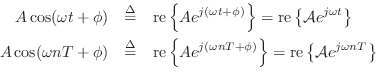
Phasor Notation
The complex amplitude
![]() is also defined as the
phasor associated with any sinusoid having amplitude
is also defined as the
phasor associated with any sinusoid having amplitude ![]() and
phase
and
phase ![]() . The term ``phasor'' is more general than ``complex
amplitude'', however, because it also applies to the corresponding
real sinusoid given by the real part of Equations (1.9-1.10).
In other words, the real sinusoids
. The term ``phasor'' is more general than ``complex
amplitude'', however, because it also applies to the corresponding
real sinusoid given by the real part of Equations (1.9-1.10).
In other words, the real sinusoids
![]() and
and
![]() may be expressed as
may be expressed as
and ![]() is the associated phasor in each case. Thus, we say that
the phasor representation of
is the associated phasor in each case. Thus, we say that
the phasor representation of
![]() is
is
![]() . Phasor analysis is
often used to analyze linear time-invariant systems such as analog
electrical circuits.
. Phasor analysis is
often used to analyze linear time-invariant systems such as analog
electrical circuits.
Plotting Complex Sinusoids as Circular Motion
Figure 1.8 shows Euler's relation graphically as it applies to
sinusoids. A point traveling with uniform velocity around a circle
with radius 1 may be represented by
![]() in
the complex plane, where
in
the complex plane, where ![]() is time and
is time and ![]() is the number of
revolutions per second. The projection of this motion onto the
horizontal (real) axis is
is the number of
revolutions per second. The projection of this motion onto the
horizontal (real) axis is
![]() , and the projection onto
the vertical (imaginary) axis is
, and the projection onto
the vertical (imaginary) axis is
![]() . For
discrete-time circular motion, replace
. For
discrete-time circular motion, replace ![]() by
by ![]() to get
to get
![]() which may be interpreted as a
point which jumps an arc length
which may be interpreted as a
point which jumps an arc length
![]() radians along the circle
each sampling instant.
radians along the circle
each sampling instant.
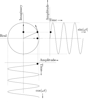 |
For circular motion to ensue, the sinusoidal motions must be at the same frequency, one-quarter cycle out of phase, and perpendicular (orthogonal) to each other. (With phase differences other than one-quarter cycle, the motion is generally elliptical.)
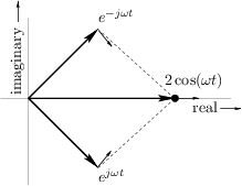
The converse of this is also illuminating. Take the usual circular
motion
![]() which spins counterclockwise along the unit
circle as
which spins counterclockwise along the unit
circle as ![]() increases, and add to it a similar but clockwise
circular motion
increases, and add to it a similar but clockwise
circular motion
![]() . This is shown in
Fig.1.9. Next apply Euler's identity to get
. This is shown in
Fig.1.9. Next apply Euler's identity to get
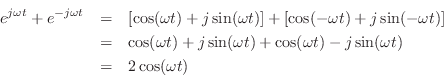
Thus,
This statement is a graphical or geometric interpretation of Eq.
We call
![]() a
positive-frequency sinusoidal component
when
a
positive-frequency sinusoidal component
when
![]() , and
, and
![]() is the
corresponding negative-frequency component. Note that both
sine and cosine signals have equal-amplitude positive- and
negative-frequency components (see also [84,53]). This
happens to be true of every real signal (i.e., non-complex). To
see this, recall that every signal can be represented as a sum of
complex sinusoids at various frequencies (its Fourier
expansion). For the signal to be real, every positive-frequency
complex sinusoid must be summed with a negative-frequency sinusoid of
equal amplitude. In other words, any counterclockwise circular motion
must be matched by an equal and opposite clockwise circular motion in
order that the imaginary parts always cancel to yield a real signal
(see Fig.1.9). Thus, a real signal always has a magnitude
spectrum which is symmetric about 0 Hz. Fourier symmetries such as
this are developed more completely in [84].
is the
corresponding negative-frequency component. Note that both
sine and cosine signals have equal-amplitude positive- and
negative-frequency components (see also [84,53]). This
happens to be true of every real signal (i.e., non-complex). To
see this, recall that every signal can be represented as a sum of
complex sinusoids at various frequencies (its Fourier
expansion). For the signal to be real, every positive-frequency
complex sinusoid must be summed with a negative-frequency sinusoid of
equal amplitude. In other words, any counterclockwise circular motion
must be matched by an equal and opposite clockwise circular motion in
order that the imaginary parts always cancel to yield a real signal
(see Fig.1.9). Thus, a real signal always has a magnitude
spectrum which is symmetric about 0 Hz. Fourier symmetries such as
this are developed more completely in [84].
Rederiving the Frequency Response
Let's repeat the mathematical sine-wave analysis of the simplest
low-pass filter, but this time using a complex sinusoid instead of a
real one. Thus, we will test the filter's response at frequency ![]() by setting its input to
by setting its input to
Using the normal rules for manipulating exponents, we find that the
output of the simple low-pass filter in response to the complex
sinusoid at frequency
![]() Hz is given by
Hz is given by
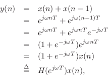
where we have defined
![]() , which we
will show is in fact the frequency response of this filter at
frequency
, which we
will show is in fact the frequency response of this filter at
frequency ![]() . This derivation is clearly easier than the
trigonometry approach. What may be puzzling at first, however, is
that the filter is expressed as a frequency-dependent complex
multiply (when the input signal is a complex sinusoid). What does
this mean? Well, the theory we are blindly trusting at this point
says it must somehow mean a gain scaling and a phase shift. This is
true and easy to see once the complex filter gain is expressed in
polar form,
. This derivation is clearly easier than the
trigonometry approach. What may be puzzling at first, however, is
that the filter is expressed as a frequency-dependent complex
multiply (when the input signal is a complex sinusoid). What does
this mean? Well, the theory we are blindly trusting at this point
says it must somehow mean a gain scaling and a phase shift. This is
true and easy to see once the complex filter gain is expressed in
polar form,
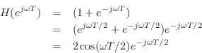
It is now easy to see that
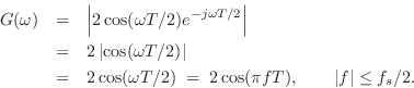
and

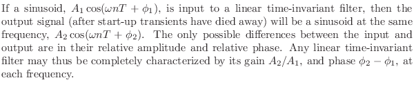
It deserves to be emphasized that all a linear time-invariant filter
can do to a sinusoid is scale its amplitude and change
its phase. Since a sinusoid is completely determined by its amplitude
![]() , frequency
, frequency ![]() , and phase
, and phase ![]() , the constraint on the filter is
that the output must also be a sinusoid, and furthermore it must be at
the same frequency as the input sinusoid. More explicitly:
, the constraint on the filter is
that the output must also be a sinusoid, and furthermore it must be at
the same frequency as the input sinusoid. More explicitly:
Mathematically, a sinusoid has no beginning and no end, so there really are no start-up transients in the theoretical setting. However, in practice, we must approximate eternal sinusoids with finite-time sinusoids whose starting time was so long ago that the filter output is essentially the same as if the input had been applied forever.
Tying it all together, the general output of a linear time-invariant filter with a complex sinusoidal input may be expressed as
![\begin{eqnarray*}
y(n) &=& (\textit{Complex Filter Gain}) \;\textit{times}\;\, (...
...ith Radius $[G(\omega)A]$\ and Phase $[\phi + \Theta(\omega)]$}.
\end{eqnarray*}](http://www.dsprelated.com/josimages_new/filters/img241.png)
Next Section:
Summary
Previous Section:
Finding the Frequency Response


