


Pole-Zero Analysis
Since our example transfer function
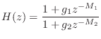

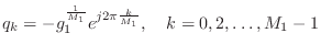
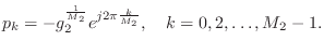
Figure 3.12 gives the pole-zero diagram of the specific example filter
![]() . There are three zeros,
marked by `O' in the figure, and five poles, marked by
`X'. Because of the simple form of digital comb filters, the
zeros (roots of
. There are three zeros,
marked by `O' in the figure, and five poles, marked by
`X'. Because of the simple form of digital comb filters, the
zeros (roots of ![]() ) are located at 0.5 times the three cube
roots of -1 (
) are located at 0.5 times the three cube
roots of -1 (
![]() ), and similarly the poles (roots
of
), and similarly the poles (roots
of ![]() ) are located at 0.9 times the five 5th roots of -1
(
) are located at 0.9 times the five 5th roots of -1
(
![]() ). (Technically, there are also two more
zeros at
). (Technically, there are also two more
zeros at ![]() .) The matlab code for producing this figure is simply
.) The matlab code for producing this figure is simply
[zeros, poles, gain] = tf2zp(B,A); % Matlab or Octave
zplane(zeros,poles); % Matlab Signal Processing Toolbox
                     % or Octave Forge
where B and A are as given in Fig.3.11. The pole-zero plot utility zplane is contained in the Matlab Signal Processing Toolbox, and in the Octave Forge collection. A similar plot is produced by
sys = tf2sys(B,A,1);
pzmap(sys);
where these functions are both in the Matlab Control Toolbox and in Octave. (Octave includes its own control-systems tool-box functions in the base Octave distribution.)
![\includegraphics[width=\twidth]{eps/epz}](http://www.dsprelated.com/josimages_new/filters/img353.png)
Next Section:
Alternative Realizations
Previous Section:
Phase Response


