


Alternative Realizations
For actually implementing the example digital filter, we have only seen the difference equation
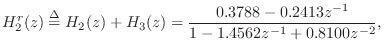
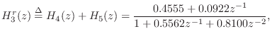
We will now illustrate the computation of a parallel second-order
realization of our example filter
![]() . As discussed above in §3.11, this filter has five
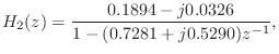
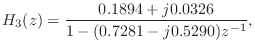
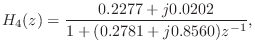
poles and three zeros. We can use the partial fraction
expansion (PFE), described in §6.8, to expand the transfer
function into a sum of five first-order terms:
. As discussed above in §3.11, this filter has five
poles and three zeros. We can use the partial fraction
expansion (PFE), described in §6.8, to expand the transfer
function into a sum of five first-order terms:
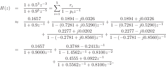
where, in the last step, complex-conjugate one-pole sections are
combined into real second-order sections. Also, numerical values are
given to four decimal places (so `![]() ' is replaced by `
' is replaced by `![]() ' in
the second line). In the following subsections, we will plot the
impulse responses and frequency responses of the first- and
second-order filter sections above.
' in
the second line). In the following subsections, we will plot the
impulse responses and frequency responses of the first- and
second-order filter sections above.
First-Order Parallel Sections
Figure 3.13 shows the impulse response of the real one-pole section
![\includegraphics[width=\twidth]{eps/arir1}](http://www.dsprelated.com/josimages_new/filters/img359.png)
![\includegraphics[width=\twidth]{eps/arfr1}](http://www.dsprelated.com/josimages_new/filters/img360.png)
Figure 3.15 shows the impulse response of the complex one-pole section
![\includegraphics[width=\twidth]{eps/arcir2}](http://www.dsprelated.com/josimages_new/filters/img362.png) |
![\includegraphics[width=\twidth]{eps/arcfr2}](http://www.dsprelated.com/josimages_new/filters/img363.png)
The complex-conjugate section,
![\includegraphics[width=\twidth]{eps/arcir3}](http://www.dsprelated.com/josimages_new/filters/img365.png) |
![\includegraphics[width=\twidth]{eps/arcfr3}](http://www.dsprelated.com/josimages_new/filters/img366.png)
Figure 3.19 shows the impulse response of the complex one-pole section
![\includegraphics[width=\twidth]{eps/arcir4}](http://www.dsprelated.com/josimages_new/filters/img371.png) |
![\includegraphics[width=\twidth]{eps/arcfr4}](http://www.dsprelated.com/josimages_new/filters/img372.png)
Parallel, Real, Second-Order Sections
Figure 3.21 shows the impulse response of the real two-pole section
![\includegraphics[width=\twidth]{eps/arir2}](http://www.dsprelated.com/josimages_new/filters/img375.png) |
![\includegraphics[width=\twidth]{eps/arfr2}](http://www.dsprelated.com/josimages_new/filters/img376.png)
Finally, Fig.3.23 gives the impulse response of the real two-pole section
![\includegraphics[width=\twidth]{eps/arir3}](http://www.dsprelated.com/josimages_new/filters/img378.png) |
![\includegraphics[width=\twidth]{eps/arfr3}](http://www.dsprelated.com/josimages_new/filters/img379.png)
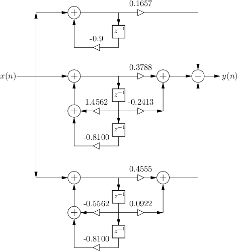
Parallel Second-Order Signal Flow Graph
Figure 3.25 shows the signal flow graph for the implementation of our
example filter using parallel second-order sections (with one
first-order section since the number of poles is odd). This is the
same filter as that shown in Fig.3.1 with ![]() ,
,
![]() ,
, ![]() , and
, and ![]() . The second-order sections are
special cases of the ``biquad'' filter section, which is often
implemented in software (and chip) libraries. Any digital filter can
be implemented as a sum of parallel biquads by finding its transfer
function and computing the partial fraction expansion.
. The second-order sections are
special cases of the ``biquad'' filter section, which is often
implemented in software (and chip) libraries. Any digital filter can
be implemented as a sum of parallel biquads by finding its transfer
function and computing the partial fraction expansion.
 |
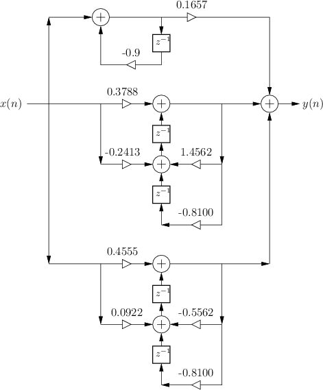 |
The two second-order biquad sections in Fig.3.25 are in so-called ``Direct-Form II'' (DF-II) form. In Chapter 9, a total of four direct-form filter implementations will be discussed, along with some other commonly used implementation structures. In particular, it is explained there why Transposed Direct-Form II (TDF-II) is usually a better choice of implementation structure for IIR filters when numerical dynamic range is limited (as it is in fixed-point ``DSP chips''). Figure 3.26 shows how our example looks using TDF-II biquads in place of the DF-II biquads of Fig.3.25.
Series, Real, Second-Order Sections
Converting the difference equation
![]() to a series bank of real first- and second-order
sections is comparatively easy. In this case, we do not need a full
blown partial fraction expansion. Instead, we need only factor the
numerator and denominator of the transfer function into first- and/or
second-order terms. Since a second-order section can accommodate up
to two poles and two zeros, we must decide how to group pairs of poles
with pairs of zeros. Furthermore, since the series sections can be
implemented in any order, we must choose the section ordering. Both
of these choices are normally driven in practice by numerical
considerations. In fixed-point implementations, the poles and zeros
are grouped such that dynamic range requirements are minimized.
Similarly, the section order is chosen so that the intermediate
signals are well scaled. For example, internal overflow is more likely
if all of the large-gain sections appear before the low-gain sections.
On the other hand, the signal-to-quantization-noise ratio will
deteriorate if all of the low-gain sections are placed before the
higher-gain sections. For further reading on numerical considerations
for digital filter sections, see, e.g., [103].
to a series bank of real first- and second-order
sections is comparatively easy. In this case, we do not need a full
blown partial fraction expansion. Instead, we need only factor the
numerator and denominator of the transfer function into first- and/or
second-order terms. Since a second-order section can accommodate up
to two poles and two zeros, we must decide how to group pairs of poles
with pairs of zeros. Furthermore, since the series sections can be
implemented in any order, we must choose the section ordering. Both
of these choices are normally driven in practice by numerical
considerations. In fixed-point implementations, the poles and zeros
are grouped such that dynamic range requirements are minimized.
Similarly, the section order is chosen so that the intermediate
signals are well scaled. For example, internal overflow is more likely
if all of the large-gain sections appear before the low-gain sections.
On the other hand, the signal-to-quantization-noise ratio will
deteriorate if all of the low-gain sections are placed before the
higher-gain sections. For further reading on numerical considerations
for digital filter sections, see, e.g., [103].
Next Section:
Summary
Previous Section:
Pole-Zero Analysis


