


Repeated Poles
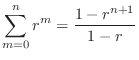
When poles are repeated, an interesting new phenomenon emerges. To see what's going on, let's consider two identical poles arranged in parallel and in series. In the parallel case, we have
Dealing with Repeated Poles Analytically
A pole of multiplicity ![]() has
has
![]() residues associated with it. For example,
residues associated with it. For example,
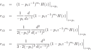
and the three residues associated with the pole
Let ![]() denote the
denote the ![]() th residue associated with the pole
th residue associated with the pole ![]() ,
,
![]() .
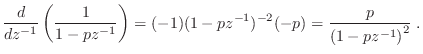
Successively differentiating
.
Successively differentiating
![]()
![]() times with
respect to
times with
respect to ![]() and setting
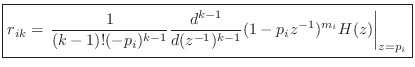
and setting ![]() isolates the residue
isolates the residue ![]() :
:
or
Example
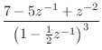
For the example of Eq.![]() (6.12), we obtain
(6.12), we obtain

Impulse Response of Repeated Poles
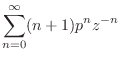
In the time domain, repeated poles give rise to polynomial amplitude envelopes on the decaying exponentials corresponding to the (stable) poles. For example, in the case of a single pole repeated twice, we have

Proof:
First note that
 |
|||
 |
|||
 |
|||
| (7.13) |
Note that
So What's Up with Repeated Poles?
In the previous section, we found that repeated poles give rise to polynomial amplitude-envelopes multiplying the exponential decay due to the pole. On the other hand, two different poles can only yield a convolution (or sum) of two different exponential decays, with no polynomial envelope allowed. This is true no matter how closely the poles come together; the polynomial envelope can occur only when the poles merge exactly. This might violate one's intuitive expectation of a continuous change when passing from two closely spaced poles to a repeated pole.
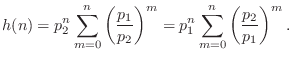
To study this phenomenon further, consider the convolution of two
one-pole impulse-responses
![]() and
and
![]() :
:
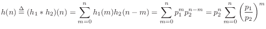
The finite limits on the summation result from the fact that both
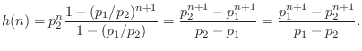
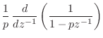
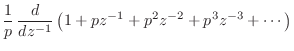
Going back to Eq.![]() (6.14), we have
(6.14), we have
 |
(7.15) |
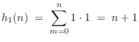
Setting
| (7.16) |
which is the first-order polynomial amplitude-envelope case for a repeated pole. We can see that the transition from ``two convolved exponentials'' to ``single exponential with a polynomial amplitude envelope'' is perfectly continuous, as we would expect.
We also see that the polynomial amplitude-envelopes fundamentally
arise from iterated convolutions. This corresponds to the
repeated poles being arranged in series, rather than in
parallel. The simplest case is when the repeated pole is at ![]() , in
which case its impulse response is a constant:
, in
which case its impulse response is a constant:

Next Section:
Alternate Stability Criterion
Previous Section:
Alternate PFE Methods


