


Similarity Transformations
A similarity transformation is a linear change of coordinates.
That is, the original ![]() -dimensional state vector
-dimensional state vector
![]() is recast
in terms of a new coordinate basis. For any linear
transformation of the coordinate basis, the transformed state vector
is recast
in terms of a new coordinate basis. For any linear
transformation of the coordinate basis, the transformed state vector
![]() may be computed by means of a matrix multiply. Denoting the
matrix of the desired one-to-one linear transformation by
may be computed by means of a matrix multiply. Denoting the
matrix of the desired one-to-one linear transformation by ![]() , we
can express the change of coordinates as
, we
can express the change of coordinates as
Let's now apply the linear transformation ![]() to the general
to the general
![]() -dimensional state-space description in Eq.
-dimensional state-space description in Eq.![]() (G.1). Substituting
(G.1). Substituting
![]() in Eq.
in Eq.![]() (G.1) gives
(G.1) gives
| (G.17) |
Premultiplying the first equation above by
| (G.18) |
Defining
we can write
| (G.20) |
The transformed system describes the same system as in Eq.
![\begin{eqnarray*}
{\tilde H}(z) &=& {\tilde D}+ {\tilde C}(zI - \tilde{A})^{-1}{...
...ht]^{-1} B\\
&=& D + C \left(zI - A\right)^{-1} B\\
&=& H(z)
\end{eqnarray*}](http://www.dsprelated.com/josimages_new/filters/img2172.png)
Since the eigenvalues of ![]() are the poles of the system, it follows
that the eigenvalues of
are the poles of the system, it follows
that the eigenvalues of
![]() are the same. In other
words, eigenvalues are unaffected by a similarity transformation. We
can easily show this directly: Let
are the same. In other
words, eigenvalues are unaffected by a similarity transformation. We
can easily show this directly: Let
![]() denote an eigenvector of
denote an eigenvector of
![]() . Then by definition
. Then by definition
![]() , where
, where ![]() is the
eigenvalue corresponding to
is the
eigenvalue corresponding to
![]() . Define
. Define
![]() as the
transformed eigenvector. Then we have
as the
transformed eigenvector. Then we have
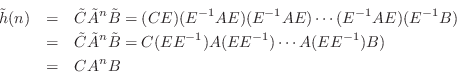
The transformed Markov parameters,
![]() , are obviously
the same also since they are given by the inverse
, are obviously
the same also since they are given by the inverse ![]() transform of the
transfer function
transform of the
transfer function
![]() . However, it is also easy to show this
by direct calculation:
. However, it is also easy to show this
by direct calculation:
Next Section:
Modal Representation
Previous Section:
Difference Equations to State Space


