


State Space Filters
An important representation for discrete-time linear systems is the state-space formulation
where
The state-space representation is especially powerful for
multi-input, multi-output (MIMO) linear systems, and also for
time-varying linear systems (in which case any or all of the matrices
in Eq.![]() (G.1) may have time subscripts
(G.1) may have time subscripts ![]() ) [37].
State-space models are also used extensively in the field of
control systems [28].
) [37].
State-space models are also used extensively in the field of
control systems [28].
An example of a Single-Input, Single-Ouput (SISO) state-space model appears in §F.6.
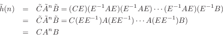
Markov Parameters
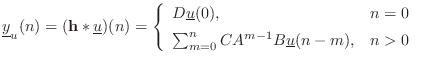
The impulse response of a state-space model is easily found by direct
calculation using Eq.![]() (G.1):
(G.1):
![\begin{eqnarray*}
\mathbf{h}(0) &=& C {\underline{x}}(0) + D\,\underline{\delta}...
... B\\ [5pt]
&\vdots&\\
\mathbf{h}(n) &=& C A^{n-1} B, \quad n>0
\end{eqnarray*}](http://www.dsprelated.com/josimages_new/filters/img2054.png)
Note that we have assumed
![]() (zero initial state or
zero initial conditions). The notation
(zero initial state or
zero initial conditions). The notation
![]() denotes a
denotes a
![]() matrix having
matrix having ![]() along the diagonal and zeros
elsewhere.G.2
along the diagonal and zeros
elsewhere.G.2
The impulse response of the state-space model can be summarized as
![$\displaystyle \fbox{$\displaystyle \mathbf{h}(n) = \left\{\begin{array}{ll} D, & n=0 \\ [5pt] CA^{n-1}B, & n>0 \\ \end{array} \right.$}$](http://www.dsprelated.com/josimages_new/filters/img2060.png) |
(G.2) |
The impulse response terms ![]() for
for ![]() are known as the
Markov parameters of the state-space model.
are known as the
Markov parameters of the state-space model.
Note that each sample of the impulse response
![]() is a
is a ![]() matrix.G.3 Therefore, it is not
a possible output signal, except when
matrix.G.3 Therefore, it is not
a possible output signal, except when ![]() . A better name might be
``impulse-matrix response''. In
§G.4 below, we'll see that
. A better name might be
``impulse-matrix response''. In
§G.4 below, we'll see that
![]() is the inverse z transform of the
matrix transfer-function of the system.
is the inverse z transform of the
matrix transfer-function of the system.
Given an arbitrary input signal
![]() (and zero intial conditions
(and zero intial conditions
![]() ), the output signal is given by the convolution of the
input signal with the impulse response:
), the output signal is given by the convolution of the
input signal with the impulse response:
Response from Initial Conditions
The response of a state-space model to initial conditions, i.e.,
its initial state
![]() is given by, again using Eq.
is given by, again using Eq.![]() (G.1),
(G.1),
Complete Response
The complete response of a linear system consists of the
superposition of (1) its response to the input signal
![]() and (2)
its response to initial conditions
and (2)
its response to initial conditions
![]() :
:
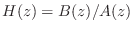
Transfer Function of a State Space Filter
The transfer function can be defined as the ![]() transform of
the impulse response:
transform of
the impulse response:
![$\displaystyle H(z) \isdef \sum_{n=0}^{\infty} h(n) z^{-n}
= D + \sum_{n=1}^{\in...
...z^{-n}
= D + z^{-1}C \left[\sum_{n=0}^{\infty} \left(z^{-1}A\right)^n\right] B
$](http://www.dsprelated.com/josimages_new/filters/img2070.png)
Note that if there are
Example State Space Filter Transfer Function
In this example, we consider a second-order filter (![]() ) with two
inputs (
) with two
inputs (![]() ) and two outputs (
) and two outputs (![]() ):
):
![\begin{eqnarray*}
A &=& g\left[\begin{array}{rr} c & -s \\ [2pt] s & c \end{arra...
... \left[\begin{array}{cc} 0 & 0 \\ [2pt] 0 & 0 \end{array}\right]
\end{eqnarray*}](http://www.dsprelated.com/josimages_new/filters/img2076.png)
so that
![\begin{eqnarray*}
\left[\begin{array}{c} x_1(n+1) \\ [2pt] x_2(n+1) \end{array}\...
...left[\begin{array}{c} x_1(n) \\ [2pt] x_2(n) \end{array}\right].
\end{eqnarray*}](http://www.dsprelated.com/josimages_new/filters/img2077.png)
From Eq.![]() (G.5), the transfer function of this MIMO digital filter is then
(G.5), the transfer function of this MIMO digital filter is then
![\begin{eqnarray*}
H(z) &=& C(zI-A)^{-1}B = (zI-A)^{-1} = \left[\begin{array}{cc}...
...z^{-2}}{\displaystyle 1-2gcz^{-1}+g^2z^{-2}} \end{array}\right].
\end{eqnarray*}](http://www.dsprelated.com/josimages_new/filters/img2078.png)
Note that when ![]() , the state transition matrix
, the state transition matrix ![]() is simply a 2D
rotation matrix, rotating through the angle
is simply a 2D
rotation matrix, rotating through the angle ![]() for which
for which
![]() and
and
![]() . For
. For ![]() , we have a type of
normalized second-order resonator [51],
and
, we have a type of
normalized second-order resonator [51],
and ![]() controls the ``damping'' of the resonator, while
controls the ``damping'' of the resonator, while
![]() controls the resonance frequency
controls the resonance frequency ![]() . The resonator
is ``normalized'' in the sense that the filter's state has a constant
. The resonator
is ``normalized'' in the sense that the filter's state has a constant
![]() norm (``preserves energy'') when
norm (``preserves energy'') when ![]() and the input is zero:
and the input is zero:
since a rotation does not change the
In this two-input, two-output digital filter, the input ![]() drives state
drives state ![]() while input
while input ![]() drives state
drives state ![]() .
Similarly, output
.
Similarly, output ![]() is
is ![]() , while
, while ![]() is
is ![]() .
The two-by-two transfer-function matrix
.
The two-by-two transfer-function matrix ![]() contains entries for
each combination of input and output. Note that all component
transfer functions have the same poles. This is a general property of
physical linear systems driven and observed at arbitrary points: the
resonant modes (poles) are always the same, but the zeros vary as the
input or output location are changed. If a pole is not visible using
a particular input/output pair, we say that the pole has been
``canceled'' by a zero associated with that input/output pair. In
control-theory terms, the pole is ``uncontrollable'' from that input,
or ``unobservable'' from that output, or both.
contains entries for
each combination of input and output. Note that all component
transfer functions have the same poles. This is a general property of
physical linear systems driven and observed at arbitrary points: the
resonant modes (poles) are always the same, but the zeros vary as the
input or output location are changed. If a pole is not visible using
a particular input/output pair, we say that the pole has been
``canceled'' by a zero associated with that input/output pair. In
control-theory terms, the pole is ``uncontrollable'' from that input,
or ``unobservable'' from that output, or both.
Transposition of a State Space Filter
Above, we found the transfer function of the general state-space model to be
When there is only one input and output signal (the SISO case), ![]() is
a scalar, as is
is
a scalar, as is ![]() . In this case we have
. In this case we have
Poles of a State Space Filter
In this section, we show that the poles of a state-space model are given
by the eigenvalues of the state-transition matrix ![]() .
.
Beginning again with the transfer function of the general state-space model,
Thus, the eigenvalues of the state transition matrix ![]() are the
poles of the corresponding linear time-invariant system. In
particular, note that the poles of the system do not depend on the
matrices
are the
poles of the corresponding linear time-invariant system. In
particular, note that the poles of the system do not depend on the
matrices ![]() , although these matrices, by placing system zeros,
can cause pole-zero cancellations (unobservable or uncontrollable
modes).
, although these matrices, by placing system zeros,
can cause pole-zero cancellations (unobservable or uncontrollable
modes).
Difference Equations to State Space
Any explicit LTI difference equation (§5.1) can be converted to state-space form. In state-space form, many properties of the system are readily obtained. For example, using standard utilities (such as in Matlab), there are functions for computing the modes of the system (its poles), an equivalent transfer-function description, stability information, and whether or not modes are ``observable'' and/or ``controllable'' from any given input/output point.
Every ![]() th order scalar (ordinary) difference equation may be reformulated
as a first order vector difference equation. For example,
consider the second-order difference equation
th order scalar (ordinary) difference equation may be reformulated
as a first order vector difference equation. For example,
consider the second-order difference equation
We may define a vector first-order difference equation--the ``state space representation''--as discussed in the following sections.
Converting to State-Space Form by Hand
Converting a digital filter to state-space form is easy because there are various ``canonical forms'' for state-space models which can be written by inspection given the strictly proper transfer-function coefficients.
The canonical forms useful for transfer-function to state-space conversion are controller canonical form (also called control or controllable canonical form) and observer canonical form (or observable canonical form) [28, p. 80], [37]. These names come from the field of control theory [28] which is concerned with designing feedback laws to control the dynamics of real-world physical systems. State-space models are used extensively in the control field to model physical systems.
The name ``controller canonical form'' reflects the fact that the
input signal can ``drive'' all modes (poles) of the system. In the
language of control theory, we may say that all of the system poles
are controllable from the input
![]() . In observer canonical form, all modes are guaranteed to be
observable. Controllability and observability of a state-space
model are discussed further in §G.7.3 below.
. In observer canonical form, all modes are guaranteed to be
observable. Controllability and observability of a state-space
model are discussed further in §G.7.3 below.
The following procedure converts any causal LTI digital filter into state-space form:
- Determine the filter transfer function
 .
.
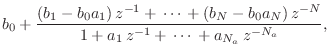
- If
 is not strictly proper (
 ),
``pull out'' the delay-free path
to obtain a feed-through gain
),
``pull out'' the delay-free path
to obtain a feed-through gain  in parallel with a strictly
proper transfer function.
in parallel with a strictly
proper transfer function.
- Write down the state-space representation by inspection using controller canonical form for the strictly proper transfer function. (Or use the matlab function tf2ss.)
We now elaborate on these steps for the general case:
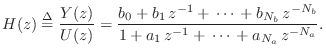
- The general causal IIR filter
has transfer function
- By convention, state-space descriptions handle any delay-free
path from input to output via the direct-path coefficient
 in
Eq.
in
Eq. (G.1). This is natural because the delay-free path does not
affect the state of the system.
(G.1). This is natural because the delay-free path does not
affect the state of the system.
A causal filter contains a delay-free path if its impulse response
 is nonzero at time zero, i.e., if
 .G.5 In such cases, we must ``pull out'' the
delay-free path in order to implement it in parallel, setting
.G.5 In such cases, we must ``pull out'' the
delay-free path in order to implement it in parallel, setting
 in the state-space model.
In our example, one step of long division yields
where , with
 for
for  , and
, and
 for
for  .
.
- The controller canonical form is then easily written as follows:
An alternate controller canonical form is obtained by applying the similarity transformation (see §G.8 below) which simply reverses the order of the state variables. Any permutation of the state variables would similarly yield a controllable form. The transpose of a controllable form is an observable form.
![\begin{displaymath}\left[
\begin{array}{ccccc}
-a_1 & -a_2 & \cdots & -a_{N-1} &...
...\ [2pt] 0 \\ [2pt] \vdots\\ [2pt] 0\end{array}\right]
\nonumber\end{displaymath}](http://www.dsprelated.com/josimages_new/filters/img2121.png)
One might worry that choosing controller canonical form may result in
unobservable modes. However, this will not happen if ![]() and
and
![]() have no common factors. In other words, if there are no
pole-zero cancellations in the transfer function
have no common factors. In other words, if there are no
pole-zero cancellations in the transfer function
![]() ,
then either controller or observer canonical form will yield a
controllable and observable state-space model.
,
then either controller or observer canonical form will yield a
controllable and observable state-space model.
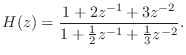
We now illustrate these steps using the example of Eq.![]() (G.7):
(G.7):
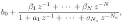
- The transfer function can be written, by inspection, as
- We need to convert Eq.(G.13) to the form
Obtaining a common denominator and equating numerator coefficients with Eq.(G.13) yields
The same result is obtained using long division (or synthetic division). - Finally, the controller canonical form is given by
![$\displaystyle \left[\begin{array}{cc} -\frac{1}{2} & -\frac{1}{3} \\ [2pt] 1 & 0 \end{array}\right]$](http://www.dsprelated.com/josimages_new/filters/img2132.png)
Converting Signal Flow Graphs to State-Space Form by Hand
The procedure of the previous section quickly converts any transfer function to state-space form (specifically, controller canonical form). When the starting point is instead a signal flow graph, it is usually easier to go directly to state-space form by labeling each delay-element output as a state variable and writing out the state-space equations by inspection of the flow graph.
For the example of the previous section, suppose we are given
Eq.![]() (G.14) in direct-form II (DF-II), as shown in
Fig.G.1. It is important that the filter representation be
canonical with respect to delay, i.e., that the number of
delay elements equals the order of the filter. Then the third step
(writing down controller canonical form by inspection) may replaced by the
following more general procedure:
(G.14) in direct-form II (DF-II), as shown in
Fig.G.1. It is important that the filter representation be
canonical with respect to delay, i.e., that the number of
delay elements equals the order of the filter. Then the third step
(writing down controller canonical form by inspection) may replaced by the
following more general procedure:
- Assign a state variable to the output of each delay element (indicated in Fig.G.1).
- Write down the state-space representation by inspection of the flow graph.
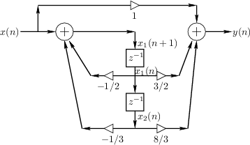 |
The state-space description of the difference equation in
Eq.![]() (G.7) is given by Eq.
(G.7) is given by Eq.![]() (G.16).
We see that controller canonical form follows immediately from the
direct-form-II digital filter realization, which is fundamentally an
all-pole filter followed by an all-zero (FIR) filter (see
§9.1.2). By starting instead from the
transposed direct-form-II (TDF-II) structure, the
observer canonical form is obtained [28, p.
87]. This is because the zeros effectively precede the
poles in a TDF-II realization, so that they may introduce nulls in the
input spectrum, but they cannot cancel output from the poles (e.g.,
from initial conditions). Since the other two digital-filter direct
forms (DF-I and TDF-I--see Chapter 9 for details) are not canonical
with respect to delay, they are not used as a basis for deriving
state-space models.
(G.16).
We see that controller canonical form follows immediately from the
direct-form-II digital filter realization, which is fundamentally an
all-pole filter followed by an all-zero (FIR) filter (see
§9.1.2). By starting instead from the
transposed direct-form-II (TDF-II) structure, the
observer canonical form is obtained [28, p.
87]. This is because the zeros effectively precede the
poles in a TDF-II realization, so that they may introduce nulls in the
input spectrum, but they cannot cancel output from the poles (e.g.,
from initial conditions). Since the other two digital-filter direct
forms (DF-I and TDF-I--see Chapter 9 for details) are not canonical
with respect to delay, they are not used as a basis for deriving
state-space models.
Controllability and Observability
Since the output ![]() in Fig.G.1 is a linear combination of
the input and states
in Fig.G.1 is a linear combination of
the input and states ![]() , one or more poles can be
canceled by the zeros induced by this linear combination. When that
happens, the canceled modes are said to be
unobservable. Of course, since we
started with a transfer function, any pole-zero cancellations should
be dealt with at that point, so that the state space realization will
always be controllable and observable. If a mode is
uncontrollable, the input cannot affect it; if it is unobservable, it
has no effect on the output. Therefore, there is usually no reason to
include unobservable or uncontrollable modes in a state-space
model.G.6
, one or more poles can be
canceled by the zeros induced by this linear combination. When that
happens, the canceled modes are said to be
unobservable. Of course, since we
started with a transfer function, any pole-zero cancellations should
be dealt with at that point, so that the state space realization will
always be controllable and observable. If a mode is
uncontrollable, the input cannot affect it; if it is unobservable, it
has no effect on the output. Therefore, there is usually no reason to
include unobservable or uncontrollable modes in a state-space
model.G.6
A physical example of uncontrollable and unobservable modes is provided by the plucked vibrating string of an electric guitar with one (very thin) magnetic pick-up. In a vibrating string, considering only one plane of vibration, each quasi-harmonicG.7 overtone corresponds to a mode of vibration [86] which may be modeled by a pair of complex-conjugate poles in a digital filter which models a particular point-to-point transfer function of the string. All modes of vibration having a node at the plucking point are uncontrollable at that point, and all modes having a node at the pick-up are unobservable at that point. If an ideal string is plucked at its midpoint, for example, all even numbered harmonics will not be excited, because they all have vibrational nodes at the string midpoint. Similarly, if the pick-up is located one-fourth of the string length from the bridge, every fourth string harmonic will be ``nulled'' in the output. This is why plucked and struck strings are generally excited near one end, and why magnetic pick-ups are located near the end of the string.
A basic result in control theory is that a system in state-space form
is controllable from a scalar input signal ![]() if and only
if the matrix
if and only
if the matrix
![\begin{displaymath}
\left[
\begin{array}{l}
C\\
CA\\
CA^2\\
\dots\\
CA^{N-1}
\end{array}\right]
\end{displaymath}](http://www.dsprelated.com/josimages_new/filters/img2142.png)
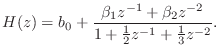
A Short-Cut to Controller Canonical Form
When converting a transfer function to state-space form by hand, the
step of pulling out the direct path, like we did in going from
Eq.![]() (G.13) to Eq.
(G.13) to Eq.![]() (G.14), can be bypassed [28, p.
87].
(G.14), can be bypassed [28, p.
87].
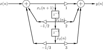 |
Figure G.2 gives the standard direct-form-II structure for a second-order
IIR filter. Unlike Fig.G.1, it includes a direct path from the
input to the output. The filter coefficients are all given directly by
the transfer function, Eq.![]() (G.13).
(G.13).
This form can be converted directly to state-space form by carefully
observing all paths from the input and state variables to the output.
For example, ![]() reaches the output through gain 2 on the right,
but also via gain
reaches the output through gain 2 on the right,
but also via gain
![]() on the left and above. Therefore, its
contribution to the output is
on the left and above. Therefore, its
contribution to the output is
![]() , as
obtained in the DF-II realization with direct-path pulled out shown in
Fig.G.1. The state variable
, as
obtained in the DF-II realization with direct-path pulled out shown in
Fig.G.1. The state variable ![]() reaches the output with
gain
reaches the output with
gain
![]() , again as we obtained before. Finally, it
must also be observed that the gain of the direct path from input to
output is
, again as we obtained before. Finally, it
must also be observed that the gain of the direct path from input to
output is ![]() .
.
Matlab Direct-Form to State-Space Conversion
Matlab and Octave support state-space models with functions such as
- tf2ss - transfer-function to state-space conversion
- ss2tf - state-space to transfer-function conversion
Let's repeat the previous example using Matlab:
>> num = [1 2 3]; % transfer function numerator
>> den = [1 1/2 1/3]; % denominator coefficients
>> [A,B,C,D] = tf2ss(num,den)

A =
   -0.5000   -0.3333
    1.0000         0

B =
     1
     0

C =  1.5000    2.6667

D =  1

>> [N,D] = ss2tf(A,B,C,D)

N = 1.0000    2.0000    3.0000

D = 1.0000    0.5000    0.3333
The tf2ss and ss2tf functions are documented online at The Mathworks help desk as well as within Matlab itself (say help tf2ss). In Octave, say help tf2ss or help -i tf2ss.
State Space Simulation in Matlab
Since matlab has first-class support for matrices and vectors, it is quite simple to implement a state-space model in Matlab using no support functions whatsoever, e.g.,
% Define the state-space system parameters:
A = [0 1; -1 0]; % State transition matrix
B = [0; 1];  C = [0 1];  D = 0; % Input, output, feed-around

% Set up the input signal, initial conditions, etc.
x0 = [0;0];             % Initial state (N=2)
Ns = 10; 	        % Number of sample times to simulate
u = [1, zeros(1,Ns-1)]; % Input signal (an impulse at time 0)
y = zeros(Ns,1);        % Preallocate output signal for n=0:Ns-1

% Perform the system simulation:
x = x0;                % Set initial state
for n=1:Ns-1           % Iterate through time
  y(n) = C*x + D*u(n); % Output for time n-1
  x = A*x + B*u(n);    % State transitions to time n
end
y' % print the output y (transposed)
% ans =
%  0   1   0  -1   0   1   0  -1   0   0
The restriction to indexes beginning at 1 is unwieldy here, because we want to include time
NUM = [0 1];
DEN = [1 0 1];
y = filter(NUM,DEN,u)
% y =
%   0   1   0  -1   0   1   0  -1   0   1
To eliminate the unit-sample delay, i.e., to simulate
[A,B,C,D] = tf2ss([1 0 0], [1 0 1])
% A =
%    0   1
%   -1  -0
%
% B =
%   0
%   1
%
% C =
%   -1   0
%
% D = 1

x = x0;                % Reset to initial state
for n=1:Ns-1
  y(n) = C*x + D*u(n);
  x = A*x + B*u(n);
end
y'
% ans =
%  1   0  -1   0   1   0  -1   0   1   0
Note the use of trailing zeros in the first argument of tf2ss (the transfer-function numerator-polynomial coefficients) to make it the same length as the second argument (denominator coefficients). This is necessary in tf2ss because the same function is used for both the continous- and discrete-time cases. Without the trailing zeros, the numerator will be extended by zeros on the left, i.e., ``right-justified'' relative to the denominator.
Other Relevant Matlab Functions
Related Signal Processing Toolbox functions include
- tf2sos --
Convert digital filter transfer function parameters to second-order
sections form. (See §9.2.)
- sos2ss --
Convert second-order filter sections to state-space form.G.8
- tf2zp --
Convert transfer-function filter parameters to zero-pole-gain form.
- ss2zp --
Convert state-space model to zeros, poles, and a gain.
- zp2ss --
Convert zero-pole-gain filter parameters to state-space form.
In Matlab, say lookfor state-space to find your state-space support utilities (there are many more than listed above). In Octave, say help -i ss2tf and keep reading for more functions (the above list is complete, as of this writing).
Matlab State-Space Filter Conversion Example
Here is the example of §F.6 repeated using matlab.G.9 The difference equation
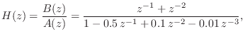
NUM = [0  1   1    0   ]; % NUM and DEN should be same length
DEN = [1 -0.5 0.1 -0.01];
The tf2ss function converts from ``transfer-function'' form to state-space form:
 [A,B,C,D] = tf2ss(NUM,DEN)
A =
   0.00000   1.00000   0.00000
   0.00000   0.00000   1.00000
   0.01000  -0.10000   0.50000

B =
  0
  0
  1

C =
  0  1  1

D = 0
Similarity Transformations
A similarity transformation is a linear change of coordinates.
That is, the original ![]() -dimensional state vector
-dimensional state vector
![]() is recast
in terms of a new coordinate basis. For any linear
transformation of the coordinate basis, the transformed state vector
is recast
in terms of a new coordinate basis. For any linear
transformation of the coordinate basis, the transformed state vector
![]() may be computed by means of a matrix multiply. Denoting the
matrix of the desired one-to-one linear transformation by
may be computed by means of a matrix multiply. Denoting the
matrix of the desired one-to-one linear transformation by ![]() , we
can express the change of coordinates as
, we
can express the change of coordinates as
Let's now apply the linear transformation ![]() to the general
to the general
![]() -dimensional state-space description in Eq.
-dimensional state-space description in Eq.![]() (G.1). Substituting
(G.1). Substituting
![]() in Eq.
in Eq.![]() (G.1) gives
(G.1) gives
| (G.17) |
Premultiplying the first equation above by
| (G.18) |
Defining
we can write
| (G.20) |
The transformed system describes the same system as in Eq.
![\begin{eqnarray*}
{\tilde H}(z) &=& {\tilde D}+ {\tilde C}(zI - \tilde{A})^{-1}{...
...ht]^{-1} B\\
&=& D + C \left(zI - A\right)^{-1} B\\
&=& H(z)
\end{eqnarray*}](http://www.dsprelated.com/josimages_new/filters/img2172.png)
Since the eigenvalues of ![]() are the poles of the system, it follows
that the eigenvalues of
are the poles of the system, it follows
that the eigenvalues of
![]() are the same. In other
words, eigenvalues are unaffected by a similarity transformation. We
can easily show this directly: Let
are the same. In other
words, eigenvalues are unaffected by a similarity transformation. We
can easily show this directly: Let
![]() denote an eigenvector of
denote an eigenvector of
![]() . Then by definition
. Then by definition
![]() , where
, where ![]() is the
eigenvalue corresponding to
is the
eigenvalue corresponding to
![]() . Define
. Define
![]() as the
transformed eigenvector. Then we have
as the
transformed eigenvector. Then we have
The transformed Markov parameters,
![]() , are obviously
the same also since they are given by the inverse
, are obviously
the same also since they are given by the inverse ![]() transform of the
transfer function
transform of the
transfer function
![]() . However, it is also easy to show this
by direct calculation:
. However, it is also easy to show this
by direct calculation:
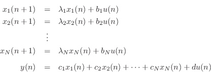
Modal Representation
When the state transition matrix ![]() is diagonal, we have the
so-called modal representation. In the single-input,
single-output (SISO) case, the general diagonal system looks like
is diagonal, we have the
so-called modal representation. In the single-input,
single-output (SISO) case, the general diagonal system looks like
![$\displaystyle \left[\begin{array}{c} x_1(n+1) \\ [2pt] x_2(n+1) \\ [2pt] \vdots \\ [2pt] x_{N-1}(n+1)\\ [2pt] x_N(n+1)\end{array}\right]$](http://www.dsprelated.com/josimages_new/filters/img2180.png)
![\begin{displaymath}\left[
\begin{array}{ccccc}
\lambda _1 & 0 & 0 & \cdots & 0 \...
...ts \\ [2pt] b_{N-1}\\ [2pt] b_N\end{array}\right] u(n)\nonumber\end{displaymath}](http://www.dsprelated.com/josimages_new/filters/img2182.png)
Since the state transition matrix is diagonal, the modes are decoupled, and we can write each mode's time-update independently:
Thus, the diagonalized state-space system consists of ![]() parallel one-pole systems. See §9.2.2
and §6.8.7 regarding the conversion of direct-form filter
transfer functions to parallel (complex) one-pole form.
parallel one-pole systems. See §9.2.2
and §6.8.7 regarding the conversion of direct-form filter
transfer functions to parallel (complex) one-pole form.
Diagonalizing a State-Space Model
To obtain the modal representation, we may diagonalize
any state-space representation. This is accomplished by means of a
particular similarity transformation specified by the
eigenvectors of the state transition matrix ![]() . An eigenvector
of the square matrix
. An eigenvector
of the square matrix ![]() is any vector
is any vector
![]() for which
for which
A system can be diagonalized whenever the eigenvectors of ![]() are
linearly independent. This always holds when the system
poles are distinct. It may or may not hold when poles are
repeated.
are
linearly independent. This always holds when the system
poles are distinct. It may or may not hold when poles are
repeated.
To see how this works, suppose we are able to find ![]() linearly
independent eigenvectors of
linearly
independent eigenvectors of ![]() , denoted
, denoted
![]() ,
,
![]() .
Then we can form an
.
Then we can form an ![]() matrix
matrix ![]() having these eigenvectors
as columns. Since the eigenvectors are linearly independent,
having these eigenvectors
as columns. Since the eigenvectors are linearly independent, ![]() is
full rank and can be used as a one-to-one linear transformation, or
change-of-coordinates matrix. From Eq.
is
full rank and can be used as a one-to-one linear transformation, or
change-of-coordinates matrix. From Eq.![]() (G.19), we have that
the transformed state transition matrix is given by
(G.19), we have that
the transformed state transition matrix is given by
![$\displaystyle \Lambda \isdef \left[\begin{array}{ccc}
\lambda_1 & & 0\\ [2pt]
& \ddots & \\ [2pt]
0 & & \lambda_N
\end{array}\right]
$](http://www.dsprelated.com/josimages_new/filters/img2193.png)
The transfer function is now, from Eq.![]() (G.5), in the SISO case,
(G.5), in the SISO case,
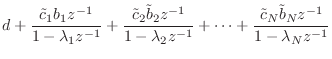

We have incidentally shown that the eigenvalues of the state-transition matrix
Notice that the diagonalized state-space form is essentially
equivalent to a partial-fraction expansion form (§6.8).
In particular, the residue of the ![]() th pole is given by
th pole is given by ![]() . When complex-conjugate poles are combined to form real,
second-order blocks (in which case
. When complex-conjugate poles are combined to form real,
second-order blocks (in which case ![]() is block-diagonal with
is block-diagonal with
![]() blocks along the diagonal), this is
corresponds to a partial-fraction expansion into real, second-order,
parallel filter sections.
blocks along the diagonal), this is
corresponds to a partial-fraction expansion into real, second-order,
parallel filter sections.
Finding the Eigenvalues of A in Practice
Small problems may be solved by hand by solving the system of equations
Example of State-Space Diagonalization
For the example of Eq.![]() (G.7), we obtain the following results:
(G.7), we obtain the following results:
>> % Initial state space filter from example above:
>> A = [-1/2, -1/3; 1, 0]; % state transition matrix
>> B = [1; 0];
>> C = [2-1/2, 3-1/3];
>> D = 1;
>>
>> eig(A) % find eigenvalues of state transition matrix A

ans =
  -0.2500 + 0.5204i
  -0.2500 - 0.5204i

>> roots(den) % find poles of transfer function H(z)

ans =
  -0.2500 + 0.5204i
  -0.2500 - 0.5204i

>> abs(roots(den)) % check stability while we're here

ans =
    0.5774
    0.5774

% The system is stable since each pole has magnitude < 1.
Our second-order example is already in real ![]() form,
because it is only second order. However, to illustrate the
computations, let's obtain the eigenvectors and compute the
complex modal representation:
form,
because it is only second order. However, to illustrate the
computations, let's obtain the eigenvectors and compute the
complex modal representation:
>> [E,L] = eig(A)  % [Evects,Evals] = eig(A)

E =

  -0.4507 - 0.2165i  -0.4507 + 0.2165i
        0 + 0.8660i        0 - 0.8660i


L =

  -0.2500 + 0.5204i        0
        0            -0.2500 - 0.5204i

>> A * E - E * L   % should be zero (A * evect = eval * evect)

ans =
  1.0e-016 *
        0 + 0.2776i        0 - 0.2776i
        0                  0

% Now form the complete diagonalized state-space model (complex):

>> Ei = inv(E); % matrix inverse
>> Ab = Ei*A*E % new state transition matrix (diagonal)

Ab =
  -0.2500 + 0.5204i   0.0000 + 0.0000i
  -0.0000            -0.2500 - 0.5204i

>> Bb = Ei*B   % vector routing input signal to internal modes

Bb =
   -1.1094
   -1.1094

>> Cb = C*E    % vector taking mode linear combination to output

Cb =
  -0.6760 + 1.9846i  -0.6760 - 1.9846i

>> Db = D      % feed-through term unchanged

Db =
     1

% Verify that we still have the same transfer function:

>> [numb,denb] = ss2tf(Ab,Bb,Cb,Db)

numb =
   1.0000             2.0000 + 0.0000i   3.0000 + 0.0000i

denb =
   1.0000             0.5000 - 0.0000i   0.3333

>> num = [1, 2, 3]; % original numerator
>> norm(num-numb)

ans =
  1.5543e-015

>> den = [1, 1/2, 1/3]; % original denominator
>> norm(den-denb)

ans =
  1.3597e-016
Properties of the Modal Representation
The vector
![]() in a modal representation (Eq.
in a modal representation (Eq.![]() (G.21)) specifies how
the modes are driven by the input. That is, the
(G.21)) specifies how
the modes are driven by the input. That is, the ![]() th mode
receives the input signal
th mode
receives the input signal ![]() weighted by
weighted by
![]() . In a computational
model of a drum, for example,
. In a computational
model of a drum, for example,
![]() may be changed corresponding to
different striking locations on the drumhead.
may be changed corresponding to
different striking locations on the drumhead.
The vector
![]() in a modal representation (Eq.
in a modal representation (Eq.![]() (G.21)) specifies how
the modes are to be mixed into the output. In other words,
(G.21)) specifies how
the modes are to be mixed into the output. In other words,
![]() specifies how the output signal is to be created as a
linear combination of the mode states:
specifies how the output signal is to be created as a
linear combination of the mode states:
The modal representation is not unique since
![]() and
and
![]() may be scaled in compensating ways to produce the same transfer
function. (The diagonal elements of
may be scaled in compensating ways to produce the same transfer
function. (The diagonal elements of ![]() may also be permuted along
with
may also be permuted along
with
![]() and
and
![]() .) Each element of the state vector
.) Each element of the state vector
![]() holds the state of a single first-order mode of the system.
holds the state of a single first-order mode of the system.
For oscillatory systems, the diagonalized state transition matrix must
contain complex elements. In particular, if mode ![]() is both
oscillatory and undamped (lossless), then an excited
state-variable
is both
oscillatory and undamped (lossless), then an excited
state-variable
![]() will oscillate sinusoidally,
after the input becomes zero, at some frequency
will oscillate sinusoidally,
after the input becomes zero, at some frequency ![]() , where
, where
In practice, we often prefer to combine complex-conjugate pole-pairs
to form a real, ``block-diagonal'' system; in this case, the
transition matrix ![]() is block-diagonal with two-by-two real matrices
along its diagonal of the form
is block-diagonal with two-by-two real matrices
along its diagonal of the form
![$\displaystyle \mathbf{A}_i = \left[\begin{array}{cc} 2R_iC_i & -R_i^2 \\ [2pt] 1 & 0 \end{array}\right]
$](http://www.dsprelated.com/josimages_new/filters/img2214.png)
Repeated Poles
The above summary of state-space diagonalization works as stated when
the modes (poles) of the system are distinct. When there are two or
more resonant modes corresponding to the same ``natural frequency''
(eigenvalue of ![]() ), then there are two further subcases: If the
eigenvectors corresponding to the repeated eigenvalue (pole) are
linearly independent, then the modes are independent and can be
treated as distinct (the system can be diagonalized). Otherwise, we
say the equal modes are coupled.
), then there are two further subcases: If the
eigenvectors corresponding to the repeated eigenvalue (pole) are
linearly independent, then the modes are independent and can be
treated as distinct (the system can be diagonalized). Otherwise, we
say the equal modes are coupled.
The coupled-repeated-poles situation is detected when the matrix of
eigenvectors V returned by the
eig matlab function [e.g., by saying
[V,D] = eig(A)] turns out to be singular.
Singularity of V can be defined as when its condition
number [cond(V)] exceeds some threshold, such as
1E7. In this case, the linearly dependent eigenvectors can
be replaced by so-called generalized eigenvectors [58].
Use of that similarity transformation then produces a ``block
diagonalized'' system instead of a diagonalized system, and one of the
blocks along the diagonal will be a ![]() matrix corresponding
to the pole repeated
matrix corresponding
to the pole repeated ![]() times.
times.
Connecting with the discussion regarding repeated poles in
§6.8.5, the ![]() Jordan block corresponding to a pole
repeated
Jordan block corresponding to a pole
repeated ![]() times plays exactly the same role of repeated poles
encountered in a partial-fraction expansion, giving rise to terms in
the impulse response proportional to
times plays exactly the same role of repeated poles
encountered in a partial-fraction expansion, giving rise to terms in
the impulse response proportional to
![]() ,
,
![]() , and so
on, up to
, and so
on, up to
![]() , where
, where ![]() denotes the repeated pole
itself (i.e., the repeated eigenvalue of the state-transition matrix
denotes the repeated pole
itself (i.e., the repeated eigenvalue of the state-transition matrix
![]() ).
).
Jordan Canonical Form
The block diagonal system having the eigenvalues along the
diagonal and ones in some of the superdiagonal elements (which serve
to couple repeated eigenvalues) is called Jordan canonical
form. Each block size corresponds to the multiplicity of the repeated
pole. As an example, a pole ![]() of multiplicity
of multiplicity ![]() could give
rise to the following
could give
rise to the following ![]() Jordan block:
Jordan block:
![$\displaystyle D_i = \left[\begin{array}{ccc}
p_i & 1 & 0\\ [2pt]
0 & p_i & 1\\ [2pt]
0 & 0 & p_i
\end{array}\right]
$](http://www.dsprelated.com/josimages_new/filters/img2223.png)
![$\displaystyle D_i = \left[\begin{array}{ccc}
p_i & 1 & 0\\ [2pt]
0 & p_i & 0\\ [2pt]
0 & 0 & p_i
\end{array}\right]
$](http://www.dsprelated.com/josimages_new/filters/img2236.png)
Interestingly, neither Matlab nor Octave seem to have a numerical function for computing the Jordan canonical form of a matrix. Matlab will try to do it symbolically when the matrix entries are given as exact rational numbers (ratios of integers) by the jordan function, which requires the Maple symbolic mathematics toolbox. Numerically, it is generally difficult to distinguish between poles that are repeated exactly, and poles that are merely close together. The residuez function sets a numerical threshold below which poles are treated as repeated.
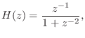
State-Space Analysis Example:
The Digital Waveguide Oscillator
As an example of state-space analysis, we will use it to determine the frequency of oscillation of the system of Fig.G.3 [90].
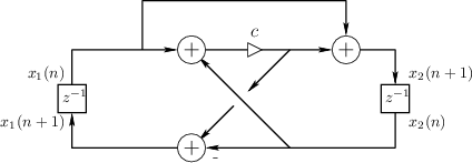
Note the assignments of unit-delay outputs to state variables ![]() and
and ![]() .
From the diagram, we see that
.
From the diagram, we see that
![$\displaystyle \left[\begin{array}{c} x_1(n+1) \\ [2pt] x_2(n+1) \end{array}\rig...
...ay}\right]}_A \left[\begin{array}{c} x_1(n) \\ [2pt] x_2(n) \end{array}\right]
$](http://www.dsprelated.com/josimages_new/filters/img2240.png)
![\begin{eqnarray*}
y_1(n) &\isdef & x_1(n) = [1, 0] {\underline{x}}(n)\\
y_2(n) &\isdef & x_2(n) = [0, 1] {\underline{x}}(n)
\end{eqnarray*}](http://www.dsprelated.com/josimages_new/filters/img2242.png)
A basic fact from linear algebra is that the determinant of a
matrix is equal to the product of its eigenvalues. As a quick
check, we find that the determinant of ![]() is
is
Note that
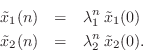
![]() . If we diagonalize this system to
obtain
. If we diagonalize this system to
obtain
![]() , where
, where
![]() diag
diag![]() ,
and
,
and ![]() is the matrix of eigenvectors of
is the matrix of eigenvectors of ![]() ,
then we have
,
then we have
![$\displaystyle \underline{{\tilde x}}(n) = \tilde{A}^n\,\underline{{\tilde x}}(0...
...t[\begin{array}{c} {\tilde x}_1(0) \\ [2pt] {\tilde x}_2(0) \end{array}\right]
$](http://www.dsprelated.com/josimages_new/filters/img2248.png)
If this system is to generate a real sampled sinusoid at radian frequency
![]() , the eigenvalues
, the eigenvalues ![]() and
and ![]() must be of the form
must be of the form
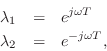
(in either order) where ![]() is real, and
is real, and ![]() denotes the sampling
interval in seconds.
denotes the sampling
interval in seconds.
Thus, we can determine the frequency of oscillation ![]() (and
verify that the system actually oscillates) by determining the
eigenvalues
(and
verify that the system actually oscillates) by determining the
eigenvalues ![]() of
of ![]() . Note that, as a prerequisite, it will
also be necessary to find two linearly independent eigenvectors of
. Note that, as a prerequisite, it will
also be necessary to find two linearly independent eigenvectors of ![]() (columns of
(columns of ![]() ).
).
Finding the Eigenstructure of A
Starting with the defining equation for an eigenvector
![]() and its
corresponding eigenvalue
and its
corresponding eigenvalue ![]() ,
,
![$\displaystyle \left[\begin{array}{cc} c & c-1 \\ [2pt] c+1 & c \end{array}\righ...
...egin{array}{c} \lambda_i \\ [2pt] \lambda_i \eta_i \end{array}\right]. \protect$](http://www.dsprelated.com/josimages_new/filters/img2255.png)
We normalized the first element of
Equation (G.23) gives us two equations in two unknowns:
Substituting the first into the second to eliminate
![\begin{eqnarray*}
1+c+c\eta_i &=& [c+\eta_i (c-1)]\eta_i = c\eta_i + \eta_i ^2 (...
...-1)\\
\,\,\Rightarrow\,\,\eta_i &=& \pm \sqrt{\frac{c+1}{c-1}}.
\end{eqnarray*}](http://www.dsprelated.com/josimages_new/filters/img2261.png)
Thus, we have found both eigenvectors
![\begin{eqnarray*}
\underline{e}_1&=&\left[\begin{array}{c} 1 \\ [2pt] \eta \end{...
...ght], \quad \hbox{where}\\
\eta&\isdef &\sqrt{\frac{c+1}{c-1}}.
\end{eqnarray*}](http://www.dsprelated.com/josimages_new/filters/img2262.png)
They are linearly independent provided
![]() and finite provided
and finite provided ![]() .
.
We can now use Eq.![]() (G.24) to find the eigenvalues:
(G.24) to find the eigenvalues:
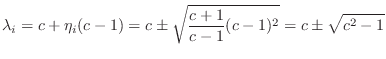
and so this is the range of
Let us henceforth assume
![]() . In this range
. In this range
![]() is real, and we have
is real, and we have
![]() ,
,
![]() . Thus, the eigenvalues can be expressed as follows:
. Thus, the eigenvalues can be expressed as follows:

Equating ![]() to
to
![]() , we obtain
, we obtain
![]() , or
, or
![]() , where
, where ![]() denotes the sampling rate. Thus the
relationship between the coefficient
denotes the sampling rate. Thus the
relationship between the coefficient ![]() in the digital waveguide
oscillator and the frequency of sinusoidal oscillation
in the digital waveguide
oscillator and the frequency of sinusoidal oscillation ![]() is
expressed succinctly as
is
expressed succinctly as
We have now shown that the system of Fig.G.3 oscillates
sinusoidally at any desired digital frequency ![]() rad/sec by simply
setting
rad/sec by simply
setting
![]() , where
, where ![]() denotes the sampling interval.
denotes the sampling interval.
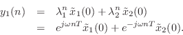
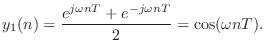
Choice of Output Signal and Initial Conditions
Recalling that
![]() , the output signal from any diagonal
state-space model is a linear combination of the modal signals. The
two immediate outputs
, the output signal from any diagonal
state-space model is a linear combination of the modal signals. The
two immediate outputs ![]() and
and ![]() in Fig.G.3 are given
in terms of the modal signals
in Fig.G.3 are given
in terms of the modal signals
![]() and
and
![]() as
as
![\begin{eqnarray*}
y_1(n) &=& [1, 0] {\underline{x}}(n) = [1, 0] \left[\begin{arr...
...\lambda_1^n {\tilde x}_1(0) - \eta \lambda_2^n\,{\tilde x}_2(0).
\end{eqnarray*}](http://www.dsprelated.com/josimages_new/filters/img2283.png)
The output signal from the first state variable ![]() is
is
The initial condition
![]() corresponds to modal initial
state
corresponds to modal initial
state
![$\displaystyle \underline{{\tilde x}}(0) = E^{-1}\left[\begin{array}{c} 1 \\ [2p...
...nd{array}\right] = \left[\begin{array}{c} 1/2 \\ [2pt] 1/2 \end{array}\right].
$](http://www.dsprelated.com/josimages_new/filters/img2286.png)
References
Further details on state-space analysis of linear systems may be found in [102,37]. More Matlab exercises and some supporting theory may be found in [10, Chapter 5].
State Space Problems
See http://ccrma.stanford.edu/~jos/filtersp/State_Space_Problems.html
Next Section:
A View of Linear Time Varying Digital Filters
Previous Section:
Matrix Filter Representations


