


Modal Representation
When the state transition matrix ![]() is diagonal, we have the
so-called modal representation. In the single-input,
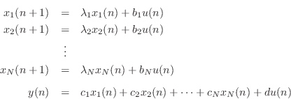
single-output (SISO) case, the general diagonal system looks like
is diagonal, we have the
so-called modal representation. In the single-input,
single-output (SISO) case, the general diagonal system looks like
![$\displaystyle \left[\begin{array}{c} x_1(n+1) \\ [2pt] x_2(n+1) \\ [2pt] \vdots \\ [2pt] x_{N-1}(n+1)\\ [2pt] x_N(n+1)\end{array}\right]$](http://www.dsprelated.com/josimages_new/filters/img2180.png)
![\begin{displaymath}\left[
\begin{array}{ccccc}
\lambda _1 & 0 & 0 & \cdots & 0 \...
...ts \\ [2pt] b_{N-1}\\ [2pt] b_N\end{array}\right] u(n)\nonumber\end{displaymath}](http://www.dsprelated.com/josimages_new/filters/img2182.png)
Since the state transition matrix is diagonal, the modes are decoupled, and we can write each mode's time-update independently:
Thus, the diagonalized state-space system consists of ![]() parallel one-pole systems. See §9.2.2
and §6.8.7 regarding the conversion of direct-form filter
transfer functions to parallel (complex) one-pole form.
parallel one-pole systems. See §9.2.2
and §6.8.7 regarding the conversion of direct-form filter
transfer functions to parallel (complex) one-pole form.
Diagonalizing a State-Space Model
To obtain the modal representation, we may diagonalize
any state-space representation. This is accomplished by means of a
particular similarity transformation specified by the
eigenvectors of the state transition matrix ![]() . An eigenvector
of the square matrix
. An eigenvector
of the square matrix ![]() is any vector
is any vector
![]() for which
for which
A system can be diagonalized whenever the eigenvectors of ![]() are
linearly independent. This always holds when the system
poles are distinct. It may or may not hold when poles are
repeated.
are
linearly independent. This always holds when the system
poles are distinct. It may or may not hold when poles are
repeated.
To see how this works, suppose we are able to find ![]() linearly
independent eigenvectors of
linearly
independent eigenvectors of ![]() , denoted
, denoted
![]() ,
,
![]() .
Then we can form an
.
Then we can form an ![]() matrix
matrix ![]() having these eigenvectors
as columns. Since the eigenvectors are linearly independent,
having these eigenvectors
as columns. Since the eigenvectors are linearly independent, ![]() is
full rank and can be used as a one-to-one linear transformation, or
change-of-coordinates matrix. From Eq.
is
full rank and can be used as a one-to-one linear transformation, or
change-of-coordinates matrix. From Eq.![]() (G.19), we have that
the transformed state transition matrix is given by
(G.19), we have that
the transformed state transition matrix is given by
![$\displaystyle \Lambda \isdef \left[\begin{array}{ccc}
\lambda_1 & & 0\\ [2pt]
& \ddots & \\ [2pt]
0 & & \lambda_N
\end{array}\right]
$](http://www.dsprelated.com/josimages_new/filters/img2193.png)
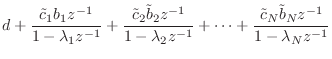
The transfer function is now, from Eq.![]() (G.5), in the SISO case,
(G.5), in the SISO case,

We have incidentally shown that the eigenvalues of the state-transition matrix
Notice that the diagonalized state-space form is essentially
equivalent to a partial-fraction expansion form (§6.8).
In particular, the residue of the ![]() th pole is given by
th pole is given by ![]() . When complex-conjugate poles are combined to form real,
second-order blocks (in which case
. When complex-conjugate poles are combined to form real,
second-order blocks (in which case ![]() is block-diagonal with
is block-diagonal with
![]() blocks along the diagonal), this is
corresponds to a partial-fraction expansion into real, second-order,
parallel filter sections.
blocks along the diagonal), this is
corresponds to a partial-fraction expansion into real, second-order,
parallel filter sections.
Finding the Eigenvalues of A in Practice
Small problems may be solved by hand by solving the system of equations
Example of State-Space Diagonalization
For the example of Eq.![]() (G.7), we obtain the following results:
(G.7), we obtain the following results:
>> % Initial state space filter from example above:
>> A = [-1/2, -1/3; 1, 0]; % state transition matrix
>> B = [1; 0];
>> C = [2-1/2, 3-1/3];
>> D = 1;
>>
>> eig(A) % find eigenvalues of state transition matrix A

ans =
  -0.2500 + 0.5204i
  -0.2500 - 0.5204i

>> roots(den) % find poles of transfer function H(z)

ans =
  -0.2500 + 0.5204i
  -0.2500 - 0.5204i

>> abs(roots(den)) % check stability while we're here

ans =
    0.5774
    0.5774

% The system is stable since each pole has magnitude < 1.
Our second-order example is already in real ![]() form,
because it is only second order. However, to illustrate the
computations, let's obtain the eigenvectors and compute the
complex modal representation:
form,
because it is only second order. However, to illustrate the
computations, let's obtain the eigenvectors and compute the
complex modal representation:
>> [E,L] = eig(A)  % [Evects,Evals] = eig(A)

E =

  -0.4507 - 0.2165i  -0.4507 + 0.2165i
        0 + 0.8660i        0 - 0.8660i


L =

  -0.2500 + 0.5204i        0
        0            -0.2500 - 0.5204i

>> A * E - E * L   % should be zero (A * evect = eval * evect)

ans =
  1.0e-016 *
        0 + 0.2776i        0 - 0.2776i
        0                  0

% Now form the complete diagonalized state-space model (complex):

>> Ei = inv(E); % matrix inverse
>> Ab = Ei*A*E % new state transition matrix (diagonal)

Ab =
  -0.2500 + 0.5204i   0.0000 + 0.0000i
  -0.0000            -0.2500 - 0.5204i

>> Bb = Ei*B   % vector routing input signal to internal modes

Bb =
   -1.1094
   -1.1094

>> Cb = C*E    % vector taking mode linear combination to output

Cb =
  -0.6760 + 1.9846i  -0.6760 - 1.9846i

>> Db = D      % feed-through term unchanged

Db =
     1

% Verify that we still have the same transfer function:

>> [numb,denb] = ss2tf(Ab,Bb,Cb,Db)

numb =
   1.0000             2.0000 + 0.0000i   3.0000 + 0.0000i

denb =
   1.0000             0.5000 - 0.0000i   0.3333

>> num = [1, 2, 3]; % original numerator
>> norm(num-numb)

ans =
  1.5543e-015

>> den = [1, 1/2, 1/3]; % original denominator
>> norm(den-denb)

ans =
  1.3597e-016
Properties of the Modal Representation
The vector
![]() in a modal representation (Eq.
in a modal representation (Eq.![]() (G.21)) specifies how
the modes are driven by the input. That is, the
(G.21)) specifies how
the modes are driven by the input. That is, the ![]() th mode
receives the input signal
th mode
receives the input signal ![]() weighted by
weighted by
![]() . In a computational
model of a drum, for example,
. In a computational
model of a drum, for example,
![]() may be changed corresponding to
different striking locations on the drumhead.
may be changed corresponding to
different striking locations on the drumhead.
The vector
![]() in a modal representation (Eq.
in a modal representation (Eq.![]() (G.21)) specifies how
the modes are to be mixed into the output. In other words,
(G.21)) specifies how
the modes are to be mixed into the output. In other words,
![]() specifies how the output signal is to be created as a
linear combination of the mode states:
specifies how the output signal is to be created as a
linear combination of the mode states:
The modal representation is not unique since
![]() and
and
![]() may be scaled in compensating ways to produce the same transfer
function. (The diagonal elements of
may be scaled in compensating ways to produce the same transfer
function. (The diagonal elements of ![]() may also be permuted along
with
may also be permuted along
with
![]() and
and
![]() .) Each element of the state vector
.) Each element of the state vector
![]() holds the state of a single first-order mode of the system.
holds the state of a single first-order mode of the system.
For oscillatory systems, the diagonalized state transition matrix must
contain complex elements. In particular, if mode ![]() is both
oscillatory and undamped (lossless), then an excited
state-variable
is both
oscillatory and undamped (lossless), then an excited
state-variable
![]() will oscillate sinusoidally,
after the input becomes zero, at some frequency
will oscillate sinusoidally,
after the input becomes zero, at some frequency ![]() , where
, where
In practice, we often prefer to combine complex-conjugate pole-pairs
to form a real, ``block-diagonal'' system; in this case, the
transition matrix ![]() is block-diagonal with two-by-two real matrices
along its diagonal of the form
is block-diagonal with two-by-two real matrices
along its diagonal of the form
![$\displaystyle \mathbf{A}_i = \left[\begin{array}{cc} 2R_iC_i & -R_i^2 \\ [2pt] 1 & 0 \end{array}\right]
$](http://www.dsprelated.com/josimages_new/filters/img2214.png)
Next Section:
Repeated Poles
Previous Section:
Similarity Transformations


