


Computation of Linear Prediction Coefficients
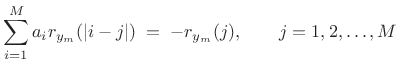
In the autocorrelation method of linear prediction, the linear
prediction coefficients
![]() are computed from the
Bartlett-window-biased autocorrelation function
(Chapter 6):
are computed from the
Bartlett-window-biased autocorrelation function
(Chapter 6):
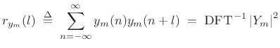
where
In matlab syntax, the solution is given by ``
If the rank of the ![]() autocorrelation matrix
autocorrelation matrix
![]() is
is ![]() , then the solution to (10.12)
is unique, and
this solution is always minimum phase [162] (i.e., all roots of
, then the solution to (10.12)
is unique, and
this solution is always minimum phase [162] (i.e., all roots of
![]() are inside the unit circle in the
are inside the unit circle in the ![]() plane [263], so
that
plane [263], so
that ![]() is always a stable all-pole filter). In
practice, the rank of
is always a stable all-pole filter). In
practice, the rank of ![]() is
is ![]() (with probability 1) whenever
(with probability 1) whenever ![]() includes a noise component. In the noiseless case, if
includes a noise component. In the noiseless case, if ![]() is a sum
of sinusoids, each (real) sinusoid at distinct frequency
is a sum
of sinusoids, each (real) sinusoid at distinct frequency
![]() adds 2 to the rank. A dc component, or a component at half the
sampling rate, adds 1 to the rank of
adds 2 to the rank. A dc component, or a component at half the
sampling rate, adds 1 to the rank of ![]() .
.
The choice of time window for forming a short-time sample
autocorrelation and its weighting also affect the rank of
![]() . Equation (10.11) applied to a finite-duration frame yields what is
called the autocorrelation method of linear
prediction [162]. Dividing out the Bartlett-window bias in such a
sample autocorrelation yields a result closer to the covariance method
of LP. A matlab example is given in §10.3.3 below.
. Equation (10.11) applied to a finite-duration frame yields what is
called the autocorrelation method of linear
prediction [162]. Dividing out the Bartlett-window bias in such a
sample autocorrelation yields a result closer to the covariance method
of LP. A matlab example is given in §10.3.3 below.
The classic covariance method computes an unbiased sample covariance
matrix by limiting the summation in (10.11) to a range over which
![]() stays within the frame--a so-called ``unwindowed'' method.
The autocorrelation method sums over the whole frame and replaces
stays within the frame--a so-called ``unwindowed'' method.
The autocorrelation method sums over the whole frame and replaces
![]() by zero when
by zero when ![]() points outside the frame--a so-called
``windowed'' method (windowed by the rectangular window).
points outside the frame--a so-called
``windowed'' method (windowed by the rectangular window).
Next Section:
Linear Prediction Order Selection
Previous Section:
Linear Prediction Methods


