


Spectrum Analysis of Noise
Spectrum analysis of noise is generally more advanced than the analysis of ``deterministic'' signals such as sinusoids, because the mathematical model for noise is a so-called stochastic process, which is defined as a sequence of random variables (see §C.1). More broadly, the analysis of signals containing noise falls under the subject of statistical signal processing [121]. Appendix C provides a short tutorial on this topic. In this chapter, we will cover only the most basic practical aspects of spectrum analysis applied to signals regarded as noise.
In particular, we will be concerned with estimating two functions from
an observed noise sequence ![]() ,
,
![]() :
:
- sample autocorrelation

- sample power spectral density (PSD)

The PSD is the Fourier transform of the autocorrelation function:
| (7.1) |
We'll accept this as nothing more than the definition of the PSD. When the signal
As indicated above, when estimating the true autocorrelation ![]() from observed samples of
from observed samples of ![]() , the resulting estimate
, the resulting estimate
![]() will
be called a sample autocorrelation. Likewise, the Fourier
transform of a sample autocorrelation will be called a sample
PSD. It is assumed that the sample PSD
will
be called a sample autocorrelation. Likewise, the Fourier
transform of a sample autocorrelation will be called a sample
PSD. It is assumed that the sample PSD
![]() converges to
the true PSD
converges to
the true PSD
![]() as
as
![]() .
.
We will also be concerned with two cases of the autocorrelation function itself:
- biased autocorrelation
- unbiased autocorrelation
 |
(7.2) |
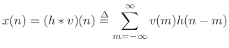
Note that this definition of autocorrelation is workable only for signals having finite support (nonzero over a finite number of samples). As shown in §2.3.7, the Fourier transform of the autocorrelation of
| (7.3) |
This chapter is concerned with noise-like signals
Since this gives an unbiased estimator of the true autocorrelation (as will be discussed below), we see that the ``bias'' in
![$\displaystyle \hat{r}_x(l) = \left\{\begin{array}{ll} \frac{(x\star x)(l)}{N-\vert l\vert}, & \vert l\vert<N \\ [5pt] 0, & \vert l\vert\ge N \\ \end{array} \right.$](http://www.dsprelated.com/josimages_new/sasp2/img1102.png) |
(7.5) |
Since the Fourier transform of a Bartlett window is
To avoid terminology confusion below, remember that the
``autocorrelation'' of a signal ![]() is defined here (and in
§2.3.7) to mean the maximally simplified case
is defined here (and in
§2.3.7) to mean the maximally simplified case
![]() , i.e., without normalization of any kind. This definition
of ``autocorrelation'' is adopted to correspond to everyday practice
in digital signal processing. The term ``sample autocorrelation'', on
the other hand, will refer to an unbiased autocorrelation
estimate. Thus, the ``autocorrelation'' of a signal
, i.e., without normalization of any kind. This definition
of ``autocorrelation'' is adopted to correspond to everyday practice
in digital signal processing. The term ``sample autocorrelation'', on
the other hand, will refer to an unbiased autocorrelation
estimate. Thus, the ``autocorrelation'' of a signal ![]() can be
viewed as a Bartlett-windowed (unbiased-)sample-autocorrelation. In the
frequency domain, the autocorrelation transforms to the
magnitude-squared Fourier transform, and the sample autocorrelation
transforms to the sample power spectral density.
can be
viewed as a Bartlett-windowed (unbiased-)sample-autocorrelation. In the
frequency domain, the autocorrelation transforms to the
magnitude-squared Fourier transform, and the sample autocorrelation
transforms to the sample power spectral density.
Introduction to Noise
Why Analyze Noise?
An example application of noise spectral analysis is denoising, in which noise is to be removed from some recording. On magnetic tape, for example, ``tape hiss'' is well modeled mathematically as a noise process. If we know the noise level in each frequency band (its power level), we can construct time-varying band gains to suppress the noise when it is audible. That is, the gain in each band is close to 1 when the music is louder than the noise, and close to 0 when the noise is louder than the music. Since tape hiss is well modeled as stationary (constant in nature over time), we can estimate the noise level during periods of ``silence'' on the tape.
Another application of noise spectral analysis is spectral modeling synthesis (the subject of §10.4). In this sound modeling technique, sinusoidal peaks are measured and removed from each frame of a short-time Fourier transform (sequence of FFTs over time). The remaining signal energy, whatever it may be, is defined as ``noise'' and resynthesized using white noise through a filter determined by the upper spectral envelope of the ``noise floor''.
What is Noise?
Consider the spectrum analysis of the following sequence:
x = [-1.55, -1.35, -0.33, -0.93, 0.39, 0.45, -0.45, -1.98]In the absence of any other information, this is just a list of numbers. It could be temperature fluctuations in some location from one day to the next, or it could be some normalization of successive samples from a music CD. There is no way to know if the numbers are ``random'' or just ``complicated''.7.2 More than a century ago, before the dawn of quantum mechanics in physics, it was thought that there was no such thing as true randomness--given the positions and momenta of all particles, the future could be predicted exactly; now, ``probability'' is a fundamental component of all elementary particle interactions in the Standard Model of physics [59].
It so happens that, in the example above, the numbers were generated by the randn function in matlab, thereby simulating normally distributed random variables with unit variance. However, this cannot be definitively inferred from a finite list of numbers. The best we can do is estimate the likelihood that these numbers were generated according to some normal distribution. The point here is that any such analysis of noise imposes the assumption that the noise data were generated by some ``random'' process. This turns out to be a very effective model for many kinds of physical processes such as thermal motions or sounds from turbulent flow. However, we should always keep in mind that any analysis we perform is carried out in terms of some underlying signal model which represents assumptions we are making regarding the nature of the data. Ultimately, we are fitting models to data.
We will consider only one type of noise: the stationary stochastic process (defined in Appendix C). All such noises can be created by passing white noise through a linear time-invariant (stable) filter [263]. Thus, for purposes of this book, the term noise always means ``filtered white noise''.
Spectral Characteristics of Noise
As we know, the spectrum ![]() of a time series
of a time series ![]() has both
a magnitude
has both
a magnitude
![]() and a phase
and a phase
![]() . The
phase of the spectrum gives information about when the signal
occurred in time. For example, if the phase is predominantly linear
with slope
. The
phase of the spectrum gives information about when the signal
occurred in time. For example, if the phase is predominantly linear
with slope ![]() , then the signal must have a prominent pulse,
onset, or other transient, at time
, then the signal must have a prominent pulse,
onset, or other transient, at time ![]() in the time domain.
in the time domain.
For stationary noise signals, the spectral phase is simply
random, and therefore devoid of information. This happens
because stationary noise signals, by definition, cannot have special
``events'' at certain times (other than their usual random
fluctuations). Thus, an important difference between the spectra of
deterministic signals (like sinusoids) and noise signals is that the
concept of phase is meaningless for noise signals. Therefore,
when we Fourier analyze a noise sequence ![]() , we will always
eliminate phase information by working with
, we will always
eliminate phase information by working with
![]() in the frequency domain (the squared-magnitude Fourier transform),
where
in the frequency domain (the squared-magnitude Fourier transform),
where
![]() .
.
White Noise
White noise may be defined as a sequence of uncorrelated random values, where correlation is defined in Appendix C and discussed further below. Perceptually, white noise is a wideband ``hiss'' in which all frequencies are equally likely. In Matlab or Octave, band-limited white noise can be generated using the rand or randn functions:
y = randn(1,100); % 100 samples of Gaussian white noise
                  % with zero mean and unit variance

x = rand(1,100);  % 100 white noise samples,
                  %   uniform between 0 and 1.
xn = 2*(x-0.5);   % Make it uniform between -1 and +1
True white noise is obtained in the limit as the sampling rate goes to infinity and as time goes to plus and minus infinity. In other words, we never work with true white noise, but rather a finite time-segment from a white noise which has been band-limited to less than half the sampling rate and sampled.
In making white noise, it doesn't matter how the amplitude values are distributed probabilistically (although that amplitude-distribution must be the same for each sample--otherwise the noise sequence would not be stationary, i.e., its statistics would be time-varying, which we exclude here). In other words, the relative probability of different amplitudes at any single sample instant does not affect whiteness, provided there is some zero-mean distribution of amplitude. It only matters that successive samples of the sequence are uncorrelated. Further discussion regarding white noise appears in §C.3.
Testing for White Noise
To test whether a set of samples can be well modeled as white noise, we may compute its sample autocorrelation and verify that it approaches an impulse in the limit as the number of samples becomes large; this is another way of saying that successive noise samples are uncorrelated. Equivalently, we may break the set of samples into successive blocks across time, take an FFT of each block, and average their squared magnitudes; if the resulting average magnitude spectrum is flat, then the set of samples looks like white noise. In the following sections, we will describe these steps in further detail, culminating in Welch's method for noise spectrum analysis, summarized in §6.9.
Sample Autocorrelation
The sample autocorrelation of a sequence ![]() ,
,
![]() may be defined by
may be defined by
where
![$\displaystyle \left\{\begin{array}{ll} \frac{1}{N-l}\sum_{n=0}^{N-1-l}\overline{v(n)}v(n+l), & l=0,1,2,\ldots,N-1 \\ [5pt] \frac{1}{N+l}\sum_{n=-l}^{N-1}\overline{v(n)}v(n+l), & l=-1,-2,\ldots,-N+1 \\ \end{array} \right. \protect$](http://www.dsprelated.com/josimages_new/sasp2/img1111.png)
and zero for
In matlab, the sample autocorrelation of a vector x can be computed using the xcorr function.7.3
Example:
octave:1> xcorr([1 1 1 1], 'unbiased')
ans =
  1   1   1   1   1   1   1
The xcorr function also performs cross-correlation when given a second signal argument, and offers additional features with additional arguments. Say help xcorr for details.
Note that
![]() is the average of the lagged product
is the average of the lagged product
![]() over all available data. For white noise, this
average approaches zero for
over all available data. For white noise, this
average approaches zero for ![]() as the number of terms in the
average increases. That is, we must have
as the number of terms in the
average increases. That is, we must have
![$\displaystyle \hat{r}_{v,N}(l) \approx \left\{\begin{array}{ll} \hat{\sigma}_{v,N}^2, & l=0 \\ [5pt] 0, & l\neq 0 \\ \end{array} \right. \isdef \hat{\sigma}_{v,N}^2 \delta(l)$](http://www.dsprelated.com/josimages_new/sasp2/img1116.png) |
(7.8) |
where
 |
(7.9) |
is defined as the sample variance of
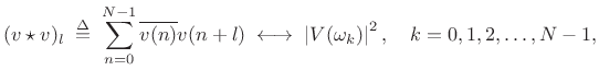
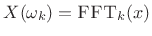
The plot in the upper left corner of Fig.6.1 shows the sample autocorrelation obtained for 32 samples of pseudorandom numbers (synthetic random numbers). (For reasons to be discussed below, the sample autocorrelation has been multiplied by a Bartlett (triangular) window.) Proceeding down the column on the left, the results of averaging many such sample autocorrelations can be seen. It is clear that the average sample autocorrelation function is approaching an impulse, as desired by definition for white noise. (The right column shows the Fourier transform of each sample autocorrelation function, which is a smoothed estimate of the power spectral density, as discussed in §6.6 below.)
![\includegraphics[width=\twidth]{eps/twhite}](http://www.dsprelated.com/josimages_new/sasp2/img1118.png)
For stationary stochastic processes ![]() , the sample autocorrelation
function
, the sample autocorrelation
function
![]() approaches the true autocorrelation function
approaches the true autocorrelation function
![]() in the limit as the number of observed samples
in the limit as the number of observed samples ![]() goes to
infinity, i.e.,
goes to
infinity, i.e.,
| (7.10) |
The true autocorrelation function of a random process is defined in Appendix C. For our purposes here, however, the above limit can be taken as the definition of the true autocorrelation function for the noise sequence
At lag ![]() , the autocorrelation function of a zero-mean random
process
, the autocorrelation function of a zero-mean random
process ![]() reduces to the variance:
reduces to the variance:
The variance can also be called the average power or mean square. The square root
Sample Power Spectral Density
The Fourier transform of the sample autocorrelation function
![]() (see (6.6)) is defined as the
sample power spectral density (PSD):
(see (6.6)) is defined as the
sample power spectral density (PSD):
 |
(7.11) |
This definition coincides with the classical periodogram when
Similarly, the true power spectral density of a stationary stochastic
processes ![]() is given by the Fourier transform of the true
autocorrelation function
is given by the Fourier transform of the true
autocorrelation function ![]() , i.e.,
, i.e.,
| (7.12) |
For real signals, the autocorrelation function is always real and
even, and therefore the power spectral density is real and even for
all real signals.
An area under the PSD,
![]() , comprises the contribution to the
variance of
, comprises the contribution to the
variance of ![]() from the frequency interval
from the frequency interval
![]() . The total integral of the PSD gives
the total variance:
. The total integral of the PSD gives
the total variance:
 |
(7.13) |
again assuming
Since the sample autocorrelation of white noise approaches an impulse, its PSD approaches a constant, as can be seen in Fig.6.1. This means that white noise contains all frequencies in equal amounts. Since white light is defined as light of all colors in equal amounts, the term ``white noise'' is seen to be analogous.
Biased Sample Autocorrelation
The sample autocorrelation defined in (6.6) is not quite
the same as the autocorrelation function for infinitely long
discrete-time sequences defined in §2.3.6,
viz.,
where the signal
Thus,
![$\displaystyle (v\star v)(l) = \left\{\begin{array}{ll} (N-\left\vert l\right\vert) \hat{r}_{v,N}(l), & l=0,\pm1,\pm2,\ldots,\pm (N-1) \\ [5pt] 0, & \vert l\vert\geq N. \\ \end{array} \right. \protect$](http://www.dsprelated.com/josimages_new/sasp2/img1137.png)
It is common in practice to retain the implicit Bartlett (triangular) weighting in the sample autocorrelation. It merely corresponds to smoothing of the power spectrum (or cross-spectrum) with the
The left column of Fig.6.1 in fact shows the Bartlett-biased sample autocorrelation. When the bias is removed, the autocorrelation appears noisier at higher lags (near the endpoints of the plot).
Smoothed Power Spectral Density
The DTFT of the Bartlett (triangular) window weighting in (6.16) is given by
![$\displaystyle N^2\cdot\hbox{asinc}^2(\omega)\isdef \left[\frac{\sin(N\omega/2)}{\sin(\omega/2)}\right]^2,$](http://www.dsprelated.com/josimages_new/sasp2/img1138.png) |
(7.17) |
where
| (7.18) |
It turns out that even more smoothing than this is essential for obtaining a stable estimate of the true PSD, as discussed further in §6.11 below.
Since the Bartlett window has no effect on an impulse signal (other than a possible overall scaling), we may use the biased autocorrelation (6.14) in place of the unbiased autocorrelation (6.15) for the purpose of testing for white noise.
The right column of Fig.6.1 shows successively greater averaging of the Bartlett-smoothed sample PSD.
Cyclic Autocorrelation
For sequences of length ![]() , the cyclic autocorrelation operator is defined by
, the cyclic autocorrelation operator is defined by
 |
(7.19) |
where
 and the index
 By using zero padding by a factor of 2 or more, cyclic autocorrelation also implements acyclic autocorrelation as defined in (6.16).
An unbiased cyclic autocorrelation is obtained, in the
zero-mean case, by simply normalizing ![]() by the number
of terms in the sum:
by the number
of terms in the sum:
 |
(7.20) |
Practical Bottom Line
Since we must use the DFT in practice, preferring an FFT for speed,
we typically compute the sample autocorrelation function for a
length ![]() sequence
sequence ![]() ,
,
![]() as follows:
as follows:
- Choose the FFT size
 to be a power of 2
providing at least
to be a power of 2
providing at least  samples of zero padding
(
samples of zero padding
(
 ):
):
![$\displaystyle x \isdef [v(0),v(1),\ldots,v(M-1), \underbrace{0,\ldots,0}_{\hbox{$N-M$}}].$](http://www.dsprelated.com/josimages_new/sasp2/img1148.png)
(7.21)
- Perform a length
FFT to get
 .
.
- Compute the squared magnitude
 .
.
- Compute the inverse FFT to get
 ,
,
 .
.
- Remove the bias, if desired, by inverting the implicit
Bartlett-window weighting to get
![$\displaystyle \hat{r}_{v,M}(l) \isdef \left\{\begin{array}{ll} \frac{1}{M-\vert l\vert} (x\star x)(l), & l=0,\,\pm1,\,\pm2,\,\pm (M-1)\;\mbox{(mod $N$)} \\ [5pt] 0, & \vert l\vert\geq M\; \mbox{(mod $N$)}. \\ \end{array} \right.$](http://www.dsprelated.com/josimages_new/sasp2/img1153.png)
(7.22)
It is important to note that the sample autocorrelation is itself a stochastic process. To stably estimate a true autocorrelation function, or its Fourier transform the power spectral density, many sample autocorrelations (or squared-magnitude FFTs) must be averaged together, as discussed in §6.12 below.
Why an Impulse is Not White Noise
Given the test for white noise that its sample autocorrelation must
approach an impulse in the limit, one might suppose that the
impulse signal ![]() is technically ``white noise'',
because its sample autocorrelation function is a perfect impulse.
However, the impulse signal fails the test of being
stationary. That is, its statistics are not the same at every
time instant. Instead, we classify an impulse as a
deterministic signal. What is true is that the impulse
signal is the deterministic counterpart of white noise. Both signals
contain all frequencies in equal amounts. We will see that all
approaches to noise spectrum analysis (that we will consider)
effectively replace noise by its autocorrelation function, thereby
converting it to deterministic form. The impulse signal is already
deterministic.
is technically ``white noise'',
because its sample autocorrelation function is a perfect impulse.
However, the impulse signal fails the test of being
stationary. That is, its statistics are not the same at every
time instant. Instead, we classify an impulse as a
deterministic signal. What is true is that the impulse
signal is the deterministic counterpart of white noise. Both signals
contain all frequencies in equal amounts. We will see that all
approaches to noise spectrum analysis (that we will consider)
effectively replace noise by its autocorrelation function, thereby
converting it to deterministic form. The impulse signal is already
deterministic.
We can modify our white-noise test to exclude obviously nonstationary
signals by dividing the signal under analysis into ![]() blocks and
computing the sample autocorrelation in each block. The final sample
autocorrelation is defined as the average of the block sample
autocorrelations. However, we can also test to see that the blocks
are sufficiently ``comparable''. A precise definition of
``comparable'' will need to wait, but intuitively, we expect that the
larger the block size (the more averaging of lagged products within
each block), the more nearly identical the results for each block
should be. For the impulse signal, the first block gives an ideal
impulse for the sample autocorrelation, while all other blocks give
the zero signal. The impulse will therefore be declared
nonstationary under any reasonable definition of what it means
to be ``comparable'' from block to block.
blocks and
computing the sample autocorrelation in each block. The final sample
autocorrelation is defined as the average of the block sample
autocorrelations. However, we can also test to see that the blocks
are sufficiently ``comparable''. A precise definition of
``comparable'' will need to wait, but intuitively, we expect that the
larger the block size (the more averaging of lagged products within
each block), the more nearly identical the results for each block
should be. For the impulse signal, the first block gives an ideal
impulse for the sample autocorrelation, while all other blocks give
the zero signal. The impulse will therefore be declared
nonstationary under any reasonable definition of what it means
to be ``comparable'' from block to block.
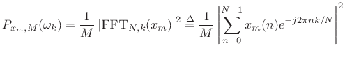
The Periodogram
The periodogram is based on the definition of the power
spectral density (PSD) (see Appendix C). Let
![]() denote a windowed segment of samples from a random process
denote a windowed segment of samples from a random process ![]() ,
where the window function
,
where the window function ![]() (classically the rectangular window)
contains
(classically the rectangular window)
contains ![]() nonzero samples. Then the periodogram is defined as the
squared-magnitude DTFT of
nonzero samples. Then the periodogram is defined as the
squared-magnitude DTFT of ![]() divided by
divided by ![]() [120, p. 65]:7.7
[120, p. 65]:7.7
In the limit as
| (7.24) |
where
In terms of the sample PSD defined in §6.7, we have
| (7.25) |
That is, the periodogram is equal to the smoothed sample PSD. In the time domain, the autocorrelation function corresponding to the periodogram is Bartlett windowed.
In practice, we of course compute a sampled periodogram
![]() ,
,
![]() , replacing the DTFT with the
length
, replacing the DTFT with the
length ![]() FFT. Essentially, the steps of §6.9
include computation of the periodogram.
FFT. Essentially, the steps of §6.9
include computation of the periodogram.
As mentioned in §6.9, a problem with the periodogram of noise
signals is that it too is random for most purposes. That is,
while the noise has been split into bands by the Fourier transform, it
has not been averaged in any way that reduces randomness, and each
band produces a nearly independent random value. In fact, it can be
shown [120] that
![]() is a random variable whose
standard deviation (square root of its variance) is comparable to its
mean.
is a random variable whose
standard deviation (square root of its variance) is comparable to its
mean.
In principle, we should be able to recover from
![]() a
filter
a
filter
![]() which, when used to filter white noise,
creates a noise indistinguishable statistically from the observed
sequence
which, when used to filter white noise,
creates a noise indistinguishable statistically from the observed
sequence ![]() . However, the DTFT is evidently useless for this
purpose. How do we proceed?
. However, the DTFT is evidently useless for this
purpose. How do we proceed?
The trick to noise spectrum analysis is that many sample power spectra (squared-magnitude FFTs) must be averaged to obtain a ``stable'' statistical estimate of the noise spectral envelope. This is the essence of Welch's method for spectrum analysis of stochastic processes, as elaborated in §6.12 below. The right column of Fig.6.1 illustrates the effect of this averaging for white noise.
Matlab for the Periodogram
Octave and the Matlab Signal Processing Toolbox have a periodogram function. Matlab for computing a periodogram of white noise is given below (see top-right plot in Fig.6.1):
M = 32;
v = randn(M,1);       % white noise
V = abs(fft(v)).^2/M; % periodogram
Welch's Method
Welch's method [296] (also called the periodogram method) for estimating power spectra is carried out by dividing the time signal into successive blocks, forming the periodogram for each block, and averaging.
Denote the ![]() th windowed, zero-padded frame from the signal
th windowed, zero-padded frame from the signal ![]() by
by
 |
(7.26) |
where
as before, and the Welch estimate of the power spectral density is given by
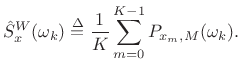
In other words, it's just an average of periodograms across time. When
Welch Autocorrelation Estimate
Since
![]() which is circular (or
cyclic) correlation, we must use zero padding in each FFT in
order to be able to compute the acyclic autocorrelation function as
the inverse DFT of the Welch PSD estimate. There is no need to
arrange the zero padding in zero-phase form, since all phase
information is discarded when the magnitude squared operation is
performed in the frequency domain.
which is circular (or
cyclic) correlation, we must use zero padding in each FFT in
order to be able to compute the acyclic autocorrelation function as
the inverse DFT of the Welch PSD estimate. There is no need to
arrange the zero padding in zero-phase form, since all phase
information is discarded when the magnitude squared operation is
performed in the frequency domain.
The Welch autocorrelation estimate is biased. That is, as
discussed in §6.6, it converges as
![]() to the true
autocorrelation
to the true
autocorrelation ![]() weighted by
weighted by ![]() (a Bartlett window). The
bias can be removed by simply dividing it out, as in
(6.15).
(a Bartlett window). The
bias can be removed by simply dividing it out, as in
(6.15).
Resolution versus Stability
A fundamental trade-off exists in Welch's method between
spectral resolution and statistical stability.
As discussed in §5.4.1, we wish to maximize the block size
![]() in order to maximize spectral resolution. On the other
hand, more blocks (larger
in order to maximize spectral resolution. On the other
hand, more blocks (larger ![]() ) gives more averaging and hence
greater spectral stability.
A typical default choice is
) gives more averaging and hence
greater spectral stability.
A typical default choice is
![]() , where
, where ![]() denotes the number of available data
samples.
denotes the number of available data
samples.
Welch's Method with Windows
As usual, the purpose of the window function ![]() (Chapter 3)
is to reduce side-lobe level in the spectral
density estimate, at the expense of frequency resolution, exactly as
in the case of sinusoidal spectrum analysis.
(Chapter 3)
is to reduce side-lobe level in the spectral
density estimate, at the expense of frequency resolution, exactly as
in the case of sinusoidal spectrum analysis.
When using a non-rectangular analysis window, the window hop-size ![]() cannot exceed half the frame length
cannot exceed half the frame length ![]() without introducing a
non-uniform sensitivity to the data
without introducing a
non-uniform sensitivity to the data ![]() over time. In the
rectangular window case, we can set
over time. In the
rectangular window case, we can set ![]() and have non-overlapping
windows. For Hamming, Hanning, and any other generalized Hamming
window, one normally sees
and have non-overlapping
windows. For Hamming, Hanning, and any other generalized Hamming
window, one normally sees ![]() for odd-length windows. For the
Blackman window,
for odd-length windows. For the
Blackman window,
![]() is typical. In general, the hop size
is typical. In general, the hop size
![]() is chosen so that the analysis window
is chosen so that the analysis window ![]() overlaps and adds
to a constant at that hop size. This consideration is explored more
fully in Chapter 8. An equivalent parameter
used by most matlab implementations is the overlap parameter
overlaps and adds
to a constant at that hop size. This consideration is explored more
fully in Chapter 8. An equivalent parameter
used by most matlab implementations is the overlap parameter
![]() .
.
Note that the number of blocks averaged in (6.27) increases
as ![]() decreases. If
decreases. If ![]() denotes the total number of signal
samples available, then the number of complete blocks available for
averaging may be computed as
denotes the total number of signal
samples available, then the number of complete blocks available for
averaging may be computed as
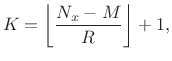 |
(7.28) |
where the floor function
Matlab for Welch's Method
Octave and the Matlab Signal Processing Toolbox have a pwelch function. Note that these functions also provide confidence intervals (not covered here). Matlab for generating the data shown in Fig.6.1 (employing Welch's method) appears in Fig.6.2.
M = 32; Ks=[1 8 32 128] nkases = length(Ks); for kase = 1:4 K = Ks(kase); N = M*K; Nfft = 2*M; % zero pad for acyclic autocorrelation Sv = zeros(Nfft,1); % PSD "accumulator" for m=1:K v = randn(M,1); % noise sample V = fft(v,Nfft); Vms = abs(V).^2; % same as conj(V) .* V Sv = Sv + Vms; % sum scaled periodograms end Sv = Sv/K; % average of all scaled periodograms rv = ifft(Sv); % Average Bartlett-windowed sample autocor. rvup = [rv(Nfft-M+1:Nfft)',rv(1:M)']; % unpack FFT rvup = rvup/M; % Normalize for no bias at lag 0 end |
Filtered White Noise
When a white-noise sequence is filtered, successive samples generally become correlated.7.8 Some of these filtered-white-noise signals have names:
- pink noise: Filter amplitude response
 is proportional to
 ; PSD
; PSD
 (``1/f noise'' -- ``equal-loudness noise'')
- brown noise: Filter amplitude response
is proportional to
 ; PSD
; PSD
 (``Brownian motion'' -- ``Wiener process'' -- ``random increments'')
In the preceding sections, we have looked at two ways of analyzing noise: the sample autocorrelation function in the time or ``lag'' domain, and the sample power spectral density (PSD) in the frequency domain. We now look at these two representations for the case of filtered noise.
Let ![]() denote a length
denote a length ![]() sequence we wish to analyze. Then the
Bartlett-windowed acyclic sample autocorrelation of
sequence we wish to analyze. Then the
Bartlett-windowed acyclic sample autocorrelation of ![]() is
is ![]() ,
and the corresponding smoothed sample PSD is
,
and the corresponding smoothed sample PSD is
![]() (§6.7, §2.3.6).
(§6.7, §2.3.6).
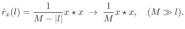
For filtered white noise, we can write ![]() as a convolution of white
noise
as a convolution of white
noise ![]() and some impulse response
and some impulse response ![]() :
:
 |
(7.29) |
The DTFT of
| (7.30) |
so that
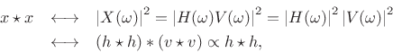
since
![]() for white noise.
Thus, we have derived that the autocorrelation of filtered white noise
is proportional to the autocorrelation of the impulse response times
the variance of the driving white noise.
for white noise.
Thus, we have derived that the autocorrelation of filtered white noise
is proportional to the autocorrelation of the impulse response times
the variance of the driving white noise.
Let's try to pin this down more precisely and find the proportionality
constant. As the number ![]() of observed samples of
of observed samples of
![]() goes to infinity, the length-
goes to infinity, the length-![]() Bartlett-window bias
Bartlett-window bias ![]() in the autocorrelation
in the autocorrelation ![]() converges to a constant scale factor
converges to a constant scale factor
![]() at lags such that
at lags such that ![]() . Therefore, the unbiased
autocorrelation can be expressed as
. Therefore, the unbiased
autocorrelation can be expressed as
 |
(7.31) |
In the limit, we obtain
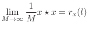 |
(7.32) |
In the frequency domain we therefore have
![\begin{eqnarray*}
S_x(\omega) &=&
\lim_{M\to \infty}\frac{1}{M}\vert X(\omega)\vert^2 \;=\;
% = \frac{1}{M}\vert H(\omega)\,V(\omega)\vert^2
\vert H(\omega)\vert^2 \cdot \lim_{M\to \infty} \frac{\vert V(\omega)\vert^2}{M} \\ [5pt]
&=&
\vert H(\omega)\vert^2 S_v(\omega) \;=\;
\vert H(\omega)\vert^2\sigma_v^2 \;\longleftrightarrow\;
(h\star h) \sigma_v^2 .
\end{eqnarray*}](http://www.dsprelated.com/josimages_new/sasp2/img1198.png)
In summary, the autocorrelation of filtered white noise ![]() is
is
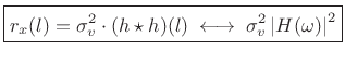 |
(7.33) |
where
In words, the true autocorrelation of filtered white noise equals the autocorrelation of the filter's impulse response times the white-noise variance. (The filter is of course assumed LTI and stable.) In the frequency domain, we have that the true power spectral density of filtered white noise is the squared-magnitude frequency response of the filter scaled by the white-noise variance.
For finite number of observed samples of a filtered white noise
process, we may say that the sample autocorrelation of filtered white
noise is given by the autocorrelation of the filter's impulse response
convolved with the sample autocorrelation of the driving white-noise
sequence. For lags ![]() much less than the number of observed samples
much less than the number of observed samples
![]() , the driver sample autocorrelation approaches an impulse scaled by
the white-noise variance. In the frequency domain, we have that the
sample PSD of filtered white noise is the squared-magnitude frequency
response of the filter
, the driver sample autocorrelation approaches an impulse scaled by
the white-noise variance. In the frequency domain, we have that the
sample PSD of filtered white noise is the squared-magnitude frequency
response of the filter
![]() scaled by a sample PSD of the
driving noise.
scaled by a sample PSD of the
driving noise.
We reiterate that every stationary random process may be defined, for our purposes, as filtered white noise.7.9 As we see from the above, all correlation information is embodied in the filter used.
Example: FIR-Filtered White Noise
Let's estimate the autocorrelation and power spectral density of the ``moving average'' (MA) process
| (7.34) |
where
Since
![]() ,
,
| (7.35) |
for nonnegative lags (
![$\displaystyle (h\star h)(l) = \left\{\begin{array}{ll} 8-l, & \vert l\vert<8 \\ [5pt] 0, & \vert l\vert\ge 8. \\ \end{array} \right.$](http://www.dsprelated.com/josimages_new/sasp2/img1206.png) |
(7.36) |
Thus, the autocorrelation of
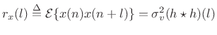 |
(7.37) |
The true power spectral density (PSD) is then
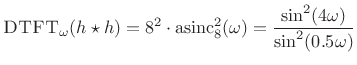 |
(7.38) |
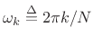
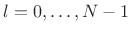
Figure 6.3 shows a collection of measured autocorrelations together with their associated smoothed-PSD estimates.
![\includegraphics[width=\twidth]{eps/tcolored}](http://www.dsprelated.com/josimages_new/sasp2/img1209.png) |
Example: Synthesis of 1/F Noise (Pink Noise)
Pink noise7.10 or
``1/f noise'' is an interesting case because it occurs often in nature
[294],7.11is often preferred by composers of computer music, and there is no
exact (rational, finite-order) filter which can produce it from
white noise. This is because the ideal amplitude response of
the filter must be proportional to the irrational function
![]() , where
, where ![]() denotes frequency in Hz. However, it is easy
enough to generate pink noise to any desired degree of approximation,
including perceptually exact.
denotes frequency in Hz. However, it is easy
enough to generate pink noise to any desired degree of approximation,
including perceptually exact.
The following Matlab/Octave code generates pretty good pink noise:
Nx = 2^16;  % number of samples to synthesize
B = [0.049922035 -0.095993537 0.050612699 -0.004408786];
A = [1 -2.494956002   2.017265875  -0.522189400];
nT60 = round(log(1000)/(1-max(abs(roots(A))))); % T60 est.
v = randn(1,Nx+nT60); % Gaussian white noise: N(0,1)
x = filter(B,A,v);    % Apply 1/F roll-off to PSD
x = x(nT60+1:end);    % Skip transient response
In the next section, we will analyze the noise produced by the above matlab and verify that its power spectrum rolls off at approximately 3 dB per octave.
Example: Pink Noise Analysis
Let's test the pink noise generation algorithm presented in
§6.14.2. We might want to know, for example, does the power
spectral density really roll off as ![]() ? Obviously such a shape
cannot extend all the way to dc, so how far does it go? Does it go
far enough to be declared ``perceptually equivalent'' to ideal 1/f
noise? Can we get by with fewer bits in the filter coefficients?
Questions like these can be answered by estimating the power spectral
density of the noise generator output.
? Obviously such a shape
cannot extend all the way to dc, so how far does it go? Does it go
far enough to be declared ``perceptually equivalent'' to ideal 1/f
noise? Can we get by with fewer bits in the filter coefficients?
Questions like these can be answered by estimating the power spectral
density of the noise generator output.
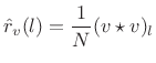
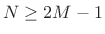
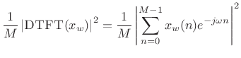
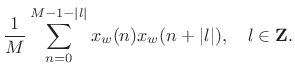
Figure 6.4 shows a single periodogram of the generated pink noise, and Figure 6.5 shows an averaged periodogram (Welch's method of smoothed power spectral density estimation). Also shown in each log-log plot is the true 1/f roll-off line. We see that indeed a single periodogram is quite random, although the overall trend is what we expect. The more stable smoothed PSD estimate from Welch's method (averaged periodograms) gives us much more confidence that the noise generator makes high quality 1/f noise.
Note that we do not have to test for stationarity in this example, because we know the signal was generated by LTI filtering of white noise. (We trust the randn function in Matlab and Octave to generate stationary white noise.)
![\includegraphics[width=\twidth]{eps/noisepr}](http://www.dsprelated.com/josimages_new/sasp2/img1210.png)
![\includegraphics[width=\twidth]{eps/noisep}](http://www.dsprelated.com/josimages_new/sasp2/img1211.png)
Processing Gain
A basic property of noise signals is that they add non-coherently. This means they sum on a
power basis instead of an amplitude basis. Thus, for
example, if you add two separate realizations of a random process
together, the total energy rises by approximately 3 dB
(
![]() ). In contrast to this, sinusoids and other
deterministic signals can add coherently. For example, at the midpoint between two
loudspeakers putting out identical signals, a sinusoidal signal is
). In contrast to this, sinusoids and other
deterministic signals can add coherently. For example, at the midpoint between two
loudspeakers putting out identical signals, a sinusoidal signal is ![]() dB louder than the signal out of each loudspeaker alone (cf.
dB louder than the signal out of each loudspeaker alone (cf. ![]() dB
for uncorrelated noise).
dB
for uncorrelated noise).
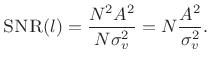
Coherent addition of sinusoids and noncoherent addition of noise can be used to obtain any desired signal to noise ratio in a spectrum analysis of sinusoids in noise. Specifically, for each doubling of the periodogram block size in Welch's method, the signal to noise ratio (SNR) increases by 3 dB (6 dB spectral amplitude increase for all sinusoids, minus 3 dB increase for the noise spectrum).
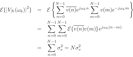
Consider a single complex sinusoid in white noise as introduced in (5.32):
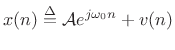 |
(7.39) |
where
![\begin{eqnarray*}
X(\omega_k)
&=& \hbox{\sc DFT}_k(x) = \sum_{n=0}^{N-1}\left[{\cal A}e^{j\omega_0 n} + v(n)\right] e^{-j\omega_k n}\\
&=& {\cal A}\sum_{n=0}^{N-1}e^{j(\omega_0 -\omega_k) n} + \sum_{n=0}^{N-1}v(n) e^{-j\omega_k n}\\
&=& {\cal A}\frac{1-e^{j(\omega_0 -\omega_k)N}}{1-e^{j(\omega_0 -\omega_k)}} + V_N(\omega_k)\\
\end{eqnarray*}](http://www.dsprelated.com/josimages_new/sasp2/img1214.png)
For simplicity, let
![]() for some
for some ![]() . That is, suppose for
now that
. That is, suppose for
now that ![]() is one of the DFT frequencies
is one of the DFT frequencies ![]() ,
,
![]() .
Then
.
Then
![\begin{eqnarray*}
X(\omega_k) &=& \left\{\begin{array}{ll}
N{\cal A}+V_N(\omega_k), & k=l \\ [5pt]
V_N(\omega_k), & k\neq l \\
\end{array} \right.\\
&=& N{\cal A}\delta(k-l)+V_N(\omega_k)
\end{eqnarray*}](http://www.dsprelated.com/josimages_new/sasp2/img1218.png)
for
![]() . Squaring the absolute value gives
. Squaring the absolute value gives
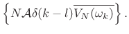 |
(7.40) |
Since
| (7.41) |
where
The final term can be expanded as
since
![]() because
because ![]() is white noise.
is white noise.
In conclusion, we have derived that the average squared-magnitude DFT
of ![]() samples of a sinusoid in white noise is given by
samples of a sinusoid in white noise is given by
| (7.42) |
where
 |
(7.43) |
In the time domain, the mean square for the signal is
Another way of viewing processing gain is to consider that the DFT
performs a change of coordinates on the observations ![]() such
that all of the signal energy ``piles up'' in one coordinate
such
that all of the signal energy ``piles up'' in one coordinate
![]() , while the noise energy remains uniformly distributed
among all of the coordinates.
, while the noise energy remains uniformly distributed
among all of the coordinates.
A practical implication of the above discussion is that it is
meaningless to quote signal-to-noise ratio in the frequency domain
without reporting the relevant bandwidth. In the above example, the
SNR could be reported as
![]() in band
in band ![]() .
.
The above analysis also makes clear the effect of bandpass
filtering on the signal-to-noise ratio (SNR). For example, consider a dc level
![]() in white noise with variance
in white noise with variance
![]() . Then the SNR
(mean-square level ratio) in the time domain is
. Then the SNR
(mean-square level ratio) in the time domain is
![]() .
Low-pass filtering at
.
Low-pass filtering at
![]() cuts the noise energy in half but
leaves the dc component unaffected, thereby increasing the SNR by
cuts the noise energy in half but
leaves the dc component unaffected, thereby increasing the SNR by
![]() dB. Each halving of the lowpass cut-off
frequency adds another 3 dB to the SNR. Since the signal is a dc
component (zero bandwidth), this process can be repeated indefinitely
to achieve any desired SNR. The narrower the lowpass filter, the
higher the SNR. Similarly, for sinusoids, the narrower the bandpass
filter centered on the sinusoid's frequency, the higher the SNR.
dB. Each halving of the lowpass cut-off
frequency adds another 3 dB to the SNR. Since the signal is a dc
component (zero bandwidth), this process can be repeated indefinitely
to achieve any desired SNR. The narrower the lowpass filter, the
higher the SNR. Similarly, for sinusoids, the narrower the bandpass
filter centered on the sinusoid's frequency, the higher the SNR.
The Panning Problem
An interesting illustration of the difference between coherent and
noncoherent signal addition comes up in the problem of stereo
panning between two loudspeakers. Let ![]() and
and ![]() denote
the signals going to the left and right loudspeakers, respectively,
and let
denote
the signals going to the left and right loudspeakers, respectively,
and let ![]() and
and ![]() denote their respective gain factors (the
``panning'' gains, between 0 and 1). When
denote their respective gain factors (the
``panning'' gains, between 0 and 1). When
![]() , sound
comes only from the left speaker, and when
, sound
comes only from the left speaker, and when
![]() , sound
comes only from the right speaker. These are the easy cases. The
harder question is what should the gains be for a sound directly in
front? It turns out that the answer depends upon the listening
geometry and the signal frequency content.
, sound
comes only from the right speaker. These are the easy cases. The
harder question is what should the gains be for a sound directly in
front? It turns out that the answer depends upon the listening
geometry and the signal frequency content.
If the listener is sitting exactly between the speakers, the ideal
``front image'' channel gains are
![]() ,
provided that the shortest wavelength in the signal is much
larger than the ear-to-ear separation of the listener. This
restriction is necessary because only those frequencies (below a few
kHz, say), will combine coherently from both speakers at each
ear. At higher frequencies, the signals from the two speakers
decorrelate at each ear because the propagation path lengths
differs significantly in units of wavelengths. (In addition, ``head
shadowing'' becomes a factor at frequencies this high.) In the
perfectly uncorrelated case (e.g., independent white noise coming from
each speaker), the energy-preserving gains are
,
provided that the shortest wavelength in the signal is much
larger than the ear-to-ear separation of the listener. This
restriction is necessary because only those frequencies (below a few
kHz, say), will combine coherently from both speakers at each
ear. At higher frequencies, the signals from the two speakers
decorrelate at each ear because the propagation path lengths
differs significantly in units of wavelengths. (In addition, ``head
shadowing'' becomes a factor at frequencies this high.) In the
perfectly uncorrelated case (e.g., independent white noise coming from
each speaker), the energy-preserving gains are
![]() . (This value is typically used in practice since the
listener may be anywhere in relation to the speakers.)
. (This value is typically used in practice since the
listener may be anywhere in relation to the speakers.)
To summarize, in ordinary stereo panning, decorrelated high
frequencies are attenuated by about 3dB, on average, when using gains
![]() dB. At any particular high frequency, the
actual gain at each ear can be anywhere between 0 and 1, but on
average, they combine on a power basis to provide a 3 dB boost on top
of the
dB. At any particular high frequency, the
actual gain at each ear can be anywhere between 0 and 1, but on
average, they combine on a power basis to provide a 3 dB boost on top
of the ![]() dB cut, leaving an overall
dB cut, leaving an overall ![]() dB change in the level at
high frequencies.
dB change in the level at
high frequencies.
Next Section:
Time-Frequency Displays
Previous Section:
Spectrum Analysis of Sinusoids


